Page 227 - Krugmans Economics for AP Text Book_Neat

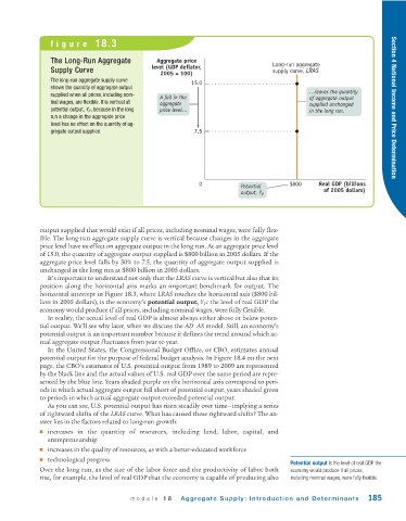
figure 18.3

The Long -Run Aggregate Aggregate price
level (GDP deflator, Long-run aggregate
Supply Curve supply curve, LRAS
2005 = 100)
The long -run aggregate supply curve
15.0
shows the quantity of aggregate output
…leaves the quantity
supplied when all prices, including nom-
A fall in the of aggregate output
inal wages, are flexible. It is vertical at aggregate supplied unchanged
potential output, Y P , because in the long price level… in the long run. Section 4 National Income and Price Determination
run a change in the aggregate price
level has no effect on the quantity of ag-
gregate output supplied. 7.5

0 Potential $800 Real GDP (billions
of 2005 dollars)
output, Y P

output supplied that would exist if all prices, including nominal wages, were fully flex-
ible. The long -run aggregate supply curve is vertical because changes in the aggregate
price level have no effect on aggregate output in the long run. At an aggregate price level
of 15.0, the quantity of aggregate output supplied is $800 billion in 2005 dollars. If the
aggregate price level falls by 50% to 7.5, the quantity of aggregate output supplied is
unchanged in the long run at $800 billion in 2005 dollars.
It’s important to understand not only that the LRAS curve is vertical but also that its
position along the horizontal axis marks an important benchmark for output. The
horizontal intercept in Figure 18.3, where LRAS touches the horizontal axis ($800 bil-
lion in 2005 dollars), is the economy’s potential output, Y P : the level of real GDP the
economy would produce if all prices, including nominal wages, were fully flexible.
In reality, the actual level of real GDP is almost always either above or below poten-
tial output. We’ll see why later, when we discuss the AD–AS model. Still, an economy’s
potential output is an important number because it defines the trend around which ac-
tual aggregate output fluctuates from year to year.
In the United States, the Congressional Budget Office, or CBO, estimates annual
potential output for the purpose of federal budget analysis. In Figure 18.4 on the next
page, the CBO’s estimates of U.S. potential output from 1989 to 2009 are represented
by the black line and the actual values of U.S. real GDP over the same period are repre-
sented by the blue line. Years shaded purple on the horizontal axis correspond to peri-
ods in which actual aggregate output fell short of potential output, years shaded green
to periods in which actual aggregate output exceeded potential output.
As you can see, U.S. potential output has risen steadily over time—implying a series
of rightward shifts of the LRAS curve. What has caused these rightward shifts? The an-
swer lies in the factors related to long -run growth:
■ increases in the quantity of resources, including land, labor, capital, and
entrepreneurship
■ increases in the quality of resources, as with a better-educated workforce
■ technological progress
Potential output is the level of real GDP the
Over the long run, as the size of the labor force and the productivity of labor both economy would produce if all prices,
rise, for example, the level of real GDP that the economy is capable of producing also including nominal wages, were fully flexible.

module 18 Aggregate Supply: Introduction and Determinants 185