Page 235 - Krugmans Economics for AP Text Book_Neat

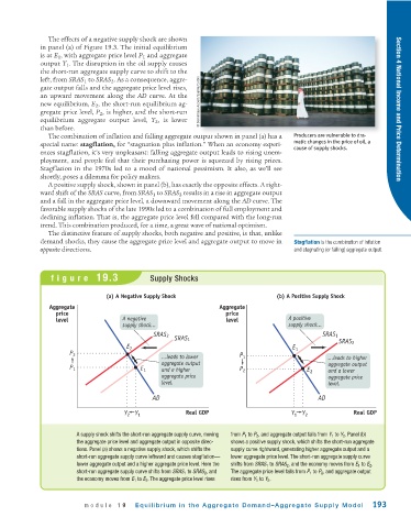
The effects of a negative supply shock are shown
in panel (a) of Figure 19.3. The initial equilibrium
is at E 1 , with aggregate price level P 1 and aggregate
output Y 1 . The disruption in the oil supply causes
the short -run aggregate supply curve to shift to the
left, from SRAS 1 to SRAS 2 . As a consequence, aggre-
gate output falls and the aggregate price level rises,
an upward movement along the AD curve. At the
new equilibrium, E 2 , the short-run equilibrium ag- © Dominique Aubert/Sygma/Corbis
gregate price level, P 2 , is higher, and the short-run Section 4 National Income and Price Determination
equilibrium aggregate output level, Y 2 , is lower
than before.
The combination of inflation and falling aggregate output shown in panel (a) has a Producers are vulnerable to dra-
special name: stagflation, for “stagnation plus inflation.” When an economy experi- matic changes in the price of oil, a
cause of supply shocks.
ences stagflation, it’s very unpleasant: falling aggregate output leads to rising unem-
ployment, and people feel that their purchasing power is squeezed by rising prices.
Stagflation in the 1970s led to a mood of national pessimism. It also, as we’ll see
shortly, poses a dilemma for policy makers.
A positive supply shock, shown in panel (b), has exactly the opposite effects. A right-
ward shift of the SRAS curve, from SRAS 1 to SRAS 2 results in a rise in aggregate output
and a fall in the aggregate price level, a downward movement along the AD curve. The
favorable supply shocks of the late 1990s led to a combination of full employment and
declining inflation. That is, the aggregate price level fell compared with the long -run
trend. This combination produced, for a time, a great wave of national optimism.
The distinctive feature of supply shocks, both negative and positive, is that, unlike
demand shocks, they cause the aggregate price level and aggregate output to move in Stagflation is the combination of inflation
opposite directions. and stagnating (or falling) aggregate output.

figure 19.3 Supply Shocks

(a) A Negative Supply Shock (b) A Positive Supply Shock
Aggregate Aggregate
price price
level A negative level A positive
supply shock... supply shock...
SRAS2 SRAS1
SRAS1
SRAS2
E 2 E 1
P 2 P
...leads to lower 1 ...leads to higher
aggregate output aggregate output
P 1 E 1 and a higher P 2 E 2 and a lower
aggregate price aggregate price
level. level.
AD AD

Y 2 Y 1 Real GDP Y 1 Y 2 Real GDP

A supply shock shifts the short -run aggregate supply curve, moving from P 1 to P 2 , and aggregate output falls from Y 1 to Y 2 . Panel (b)
the aggregate price level and aggregate output in opposite direc- shows a positive supply shock, which shifts the short -run aggregate
tions. Panel (a) shows a negative supply shock, which shifts the supply curve rightward, generating higher aggregate output and a
short -run aggregate supply curve leftward and causes stagflation— lower aggregate price level. The short -run aggregate supply curve
lower aggregate output and a higher aggregate price level. Here the shifts from SRAS 1 to SRAS 2 , and the economy moves from E 1 to E 2 .
short -run aggregate supply curve shifts from SRAS 1 to SRAS 2 , and The aggregate price level falls from P 1 to P 2 , and aggregate output
the economy moves from E 1 to E 2 . The aggregate price level rises rises from Y 1 to Y 2 .

module 19 Equilibrium in the Aggregate Demand–Aggregate Supply Model 193