Page 237 - Krugmans Economics for AP Text Book_Neat

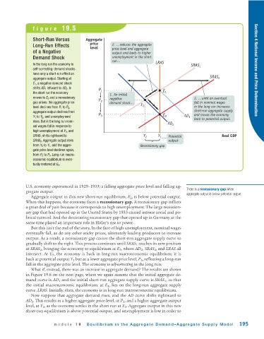
figure 19.5

Short -Run Versus Aggregate
price
Long -Run Effects 2. …reduces the aggregate
level price level and aggregate
of a Negative output and leads to higher
Demand Shock unemployment in the short
run… LRAS
In the long run the economy is
SRAS 1
self -correcting: demand shocks Section 4 National Income and Price Determination
have only a short -run effect on
aggregate output. Starting at SRAS 2
E 1 , a negative demand shock
shifts AD 1 leftward to AD 2 . In
P 1 E
the short run the economy 1
1. An initial
moves to E 2 and a recessionary negative 3. …until an eventual
P 2
gap arises: the aggregate price demand shock… fall in nominal wages
E 2
level declines from P 1 to P 2 , in the long run increases
aggregate output declines from short-run aggregate supply
Y 1 to Y 2 , and unemployment P 3 E 3 AD 1 and moves the economy
back to potential output.
rises. But in the long run nomi-
AD 2
nal wages fall in response to
high unemployment at Y 2 , and
SRAS 1 shifts rightward to Y 2 Y 1 Potential Real GDP
SRAS 2 . Aggregate output rises output
from Y 2 to Y 1 , and the aggre- Recessionary gap
gate price level declines again,
from P 2 to P 3 . Long -run macro-
economic equilibrium is even-
tually restored at E 3 .

U.S. economy experienced in 1929–1933: a falling aggregate price level and falling ag-
gregate output. There is a recessionary gap when
aggregate output is below potential output.
Aggregate output in this new short -run equilibrium, E 2 , is below potential output.
When this happens, the economy faces a recessionary gap. A recessionary gap inflicts
a great deal of pain because it corresponds to high unemployment. The large recession-
ary gap that had opened up in the United States by 1933 caused intense social and po-
litical turmoil. And the devastating recessionary gap that opened up in Germany at the
same time played an important role in Hitler’s rise to power.
But this isn’t the end of the story. In the face of high unemployment, nominal wages
eventually fall, as do any other sticky prices, ultimately leading producers to increase
output. As a result, a recessionary gap causes the short -run aggregate supply curve to
gradually shift to the right. This process continues until SRAS 1 reaches its new position
at SRAS 2 , bringing the economy to equilibrium at E 3 , where AD 2 , SRAS 2 , and LRAS all
intersect. At E 3 , the economy is back in long -run macroeconomic equilibrium; it is
back at potential output Y 1 but at a lower aggregate price level, P 3 , reflecting a long -run
fall in the aggregate price level. The economy is self -correcting in the long run.
What if, instead, there was an increase in aggregate demand? The results are shown
in Figure 19.6 on the next page, where we again assume that the initial aggregate de-
mand curve is AD 1 and the initial short -run aggregate supply curve is SRAS 1 , so that
the initial macroeconomic equilibrium, at E 1 , lies on the long -run aggregate supply
curve, LRAS. Initially, then, the economy is in long -run macroeconomic equilibrium.
Now suppose that aggregate demand rises, and the AD curve shifts rightward to
AD 2 . This results in a higher aggregate price level, at P 2 , and a higher aggregate output
level, at Y 2 , as the economy settles in the short run at E 2 . Aggregate output in this new
short -run equilibrium is above potential output, and unemployment is low in order to

module 19 Equilibrium in the Aggregate Demand–Aggregate Supply Model 195