Page 61 - Krugmans Economics for AP Text Book_Neat

Opportunity Cost

The production possibilities curve is also useful as a reminder that the true cost of
any good is not only its price, but also everything else in addition to money that
must be given up in order to get that good—the opportunity cost. If, for example, Tom
decides to go from point A to point B, he will produce 8 more fish but 6 fewer co-
conuts. So the opportunity cost of those 8 fish is the 6 coconuts not gathered. Since
8 extra fish have an opportunity cost of 6 coconuts, 1 fish has an opportunity cost Section I Basic Economic Concepts
6
3
of ⁄8 = ⁄4 of a coconut.
Is the opportunity cost of an extra fish in terms of coconuts always the same, no
matter how many fish Tom catches? In the example illustrated by Figure 3.1, the an-
swer is yes. If Tom increases his catch from 28 to 40 fish, an increase of 12, the number
of coconuts he gathers falls from 9 to zero. So his opportunity cost per additional fish
9
3
is ⁄12 = ⁄4 of a coconut, the same as it was when his catch went from 20 fish to 28. How-
ever, the fact that in this example the opportunity cost of an additional fish in terms of
coconuts is always the same is a result of an assumption we’ve made, an assumption
that’s reflected in the way Figure 3.1 is drawn. Specifically, whenever we assume that
the opportunity cost of an additional unit of a good doesn’t change regardless of the
output mix, the production possibilities curve is a straight line.
Moreover, as you might have already guessed, the slope of a straight-line production
possibilities curve is equal to the opportunity cost—specifically, the opportunity cost for
the good measured on the horizontal axis in terms of the good measured on the vertical
3
axis. In Figure 3.1, the production possibilities curve has a constant slope of − ⁄4, implying
3
that Tom faces a constant opportunity cost per fish equal to ⁄4 of a coconut. (A review of
how to calculate the slope of a straight line is found in the Section I Appendix.) This is
the simplest case, but the production possibilities curve model can also be used to ex-
amine situations in which opportunity costs change as the mix of output changes.
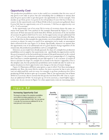
Figure 3.2 illustrates a different assumption, a case in which Tom faces increasing op-
portunity cost. Here, the more fish he catches, the more coconuts he has to give up to
catch an additional fish, and vice versa. For example, to go from producing zero fish to
producing 20 fish, he has to give up 5 coconuts. That is, the opportunity cost of those
20 fish is 5 coconuts. But to increase his fish production from 20 to 40—that is, to pro-
duce an additional 20 fish—he must give up 25 more coconuts, a much higher oppor-
tunity cost. As you can see in Figure 3.2, when opportunity costs are increasing rather

figure 3.2

Increasing Opportunity Cost Quantity
of coconuts
The bowed-out shape of the production possibilities Producing the first . . . requires giving
curve reflects increasing opportunity cost. In this 35 20 fish . . . up 5 coconuts.
example, to produce the first 20 fish, Tom must give up
5 coconuts. But to produce an additional 20 fish, he 30 But producing 20
more fish . . .
must give up 25 more coconuts. A
25
20
. . . requires
15 giving up 25
more coconuts.
10

5
PPC
0 10 20 30 40 50
Quantity of fish

module 3 The Production Possibilities Curve Model 19