Page 242 - Algorithms Notes for Professionals

Chapter 54: Dynamic Time Warping

Section 54.1: Introduction To Dynamic Time Warping

Dynamic Time Warping (DTW) is an algorithm for measuring similarity between two temporal sequences which may
vary in speed. For instance, similarities in walking could be detected using DTW, even if one person was walking
faster than the other, or if there were accelerations and decelerations during the course of an observation. It can be
used to match a sample voice command with others command, even if the person talks faster or slower than the
prerecorded sample voice. DTW can be applied to temporal sequences of video, audio and graphics data-indeed,
any data which can be turned into a linear sequence can be analyzed with DTW.

In general, DTW is a method that calculates an optimal match between two given sequences with certain
restrictions. But let's stick to the simpler points here. Let's say, we have two voice sequences Sample and Test, and
we want to check if these two sequences match or not. Here voice sequence refers to the converted digital signal of
your voice. It might be the amplitude or frequency of your voice that denotes the words you say. Let's assume:

Sample = {1, 2, 3, 5, 5, 5, 6}
Test = {1, 1, 2, 2, 3, 5}

We want to find out the optimal match between these two sequences.

At first, we define the distance between two points, d(x, y) where x and y represent the two points. Let,

d(x, y) = |x - y| //absolute difference

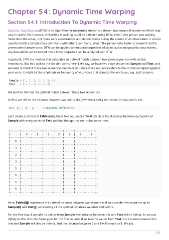
Let's create a 2D matrix Table using these two sequences. We'll calculate the distances between each point of
Sample with every points of Test and find the optimal match between them.

+------+------+------+------+------+------+------+------+
| | 0 | 1 | 1 | 2 | 2 | 3 | 5 |
+------+------+------+------+------+------+------+------+
| 0 | | | | | | | |
+------+------+------+------+------+------+------+------+
| 1 | | | | | | | |
+------+------+------+------+------+------+------+------+
| 2 | | | | | | | |
+------+------+------+------+------+------+------+------+
| 3 | | | | | | | |
+------+------+------+------+------+------+------+------+
| 5 | | | | | | | |
+------+------+------+------+------+------+------+------+
| 5 | | | | | | | |
+------+------+------+------+------+------+------+------+
| 5 | | | | | | | |
+------+------+------+------+------+------+------+------+
| 6 | | | | | | | |
+------+------+------+------+------+------+------+------+

Here, Table[i][j] represents the optimal distance between two sequences if we consider the sequence up to
Sample[i] and Test[j], considering all the optimal distances we observed before.

For the first row, if we take no values from Sample, the distance between this and Test will be infinity. So we put
infinity on the first row. Same goes for the first column. If we take no values from Test, the distance between this
one and Sample will also be infinity. And the distance between 0 and 0 will simply be 0. We get,

colegiohispanomexicano.net – Algorithms Notes 238