Page 3 - water-11-02048-v2

Water 2019, 11, 2048 3 of 14

2.1. One-Dimensional River Flow Modeling

In 1D river hydraulic modeling, all water flows are assumed to flow in a longitudinal direction.
One-dimensional models represent the terrain as a sequence of cross-sections and simulate the flow
in order to provide estimates of flow parameters such as flow velocity and water depth. To simplify
the computation, HEC-RAS assumed a horizontal water surface at each cross-section normal to the
direction of the flow such that the momentum exchange between the channel and the floodplain can be
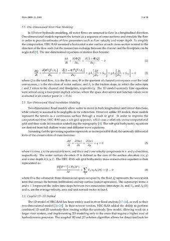
neglected [9]. The one-dimensional equations of motion then become:

∂A ∂(ΦQ) ∂[(1 − Φ)Q]
+ + = 0 (1)
∂t ∂x c ∂x f

h i
2 2 2 2 " # " #
∂Q ∂ Φ Q /A c ∂ (1 − Φ) Q /A f ∂Z ∂z
+ + + gA c + S fc + gA f + S f f = 0 (2)
∂t ∂x c ∂x f ∂x c ∂x f
where Q is the total flow, A is the flow area, Φ is the quotient of channel conveyance over the total
conveyance, z is the elevation of water surface, and S is the friction slope, in which the subscripts
f
c and f refers to the channel and floodplain, respectively. The 1D model unsteady flow equations
were solved using a four-point implicit scheme, where the space derivatives and function values were
evaluated at an interior point (n + θ)∆t.

2.2. Two-Dimensional Flood Inundation Modeling

Two-dimensional flood models allow water to move in both longitudinal and lateral directions,
while velocity is assumed to be negligible in the z-direction. However, unlike 1D models, these models
represent the terrain as a continuous surface through a mesh or grid. In order to improve the
computational time, HEC-RAS uses a sub-grid approach, which uses a relatively coarse computational
grid and finer scale information underlying the topography [9]. The sub-grid bathymetry equations
are derived from full shallow water and diffusion wave equations.
Assuming that the governing equation represents an incompressible fluid, the unsteady differential
form of the conservation of mass becomes:

∂H ∂(hu) ∂(hv)
+ + + q = 0 (3)
∂t ∂x ∂y

where t is time, q is the source/sink term, and the u and v are velocity components in x- and y-directions,
respectively. The water surface elevation H is defined as the sum of the surface elevation z(x, y)
and water depth h(x, y, t). The HEC-RAS sub-grid bathymetry mass conservation equation is then
represented as:

n
Ω H n+1 − Ω(H ) X
+ V ·n A (H) + Q = 0 (4)
k
k
k
∆t
k
where Ω is the volumetric three-dimensional space occupied by the fluid, Q represents the source/sink
term that crosses the bottom (infiltration) and top surface (rain/evaporation). The superscript terms n
and n + 1 represent the index time-steps between two consecutive time-steps ∆t, and V , and A (H)
k
k
and n are the average velocity, area and unit normal vector at face k.
k
2.3. Coupled 1D–2D Method
The 1D model of HEC-RAS has been widely used in river flood analysis [17–24], as well as their
two-dimensional model [24–28]. In their newest version, HEC-RAS added the ability to perform
combined 1D and 2D unsteady-flow routing within the unsteady flow model, allowing work on a
larger river system, and implementing 2D modeling only in the areas that require a higher level of
hydrodynamic precision. The coupled 1D and 2D solution algorithm allows for direct feedback for