Page 6 - water-11-02048-v2

Water 2019, 11, 2048 6 of 14

3.2. Methodology

In order to run the simulation for the HEC-RAS coupled 1D–2D model, the results from the
HEC-RAS one-dimensional model were used for the input data. These 1D data were also used in
previous research in simulating Baeksan flood inundation. The mesh domain for the 2D flow was set
up, as well as the lateral structure and boundary conditions. After running the simulation, the resulting
Water 2019, 11, x FOR PEER REVIEW 6 of 14
flood data—flood extent, water surface elevation, water depth, change in flooded area and flow
velocity—were mapped using the geographic information system (GIS) tool, and then compared to the
flow velocity—were mapped using the geographic information system (GIS) tool, and then compared
flood results from the observed data, Gerris and FLUMEN models. In this way, the model’s capability
to the flood results from the observed data, Gerris and FLUMEN models. In this way, the model’s
and accuracy can be assessed.
capability and accuracy can be assessed.
3.3. Pre-Simulation Conditions
3.3. Pre-Simulation Conditions
In 2D modeling, a spatial representation of flow can either be constructed through a structured
In 2D modeling, a spatial representation of flow can either be constructed through a structured
mesh (regular grid), unstructured mesh (triangular grid) or flexible mesh. However, difficulties in the
mesh (regular grid), unstructured mesh (triangular grid) or flexible mesh. However, difficulties in
simulation can be encountered in some cases where topographic data is too dense to be realistically
the simulation can be encountered in some cases where topographic data is too dense to be
used as a grid for numerical modelling. This poses challenges when a coarse grid must be used to
realistically used as a grid for numerical modelling. This poses challenges when a coarse grid must
generate an overall fluid simulation, but finer features needed to be incorporated in the computation
be used to generate an overall fluid simulation, but finer features needed to be incorporated in the
as well. To solve this problem, recent advances in two-dimensional modeling include the adaptive
computation as well. To solve this problem, recent advances in two-dimensional modeling include
mesh refinement method [6] and hybrid 1D–2D variable grid sizing technique [8]. HEC-RAS, however,
the adaptive mesh refinement method [6] and hybrid 1D–2D variable grid sizing technique [8]. HEC-
uses the sub-grid bathymetry approach, where the extra information is pre-computed from fine
RAS, however, uses the sub-grid bathymetry approach, where the extra information is pre-computed
bathymetry. The high-resolution details are neglected, but enough data are available so that the coarser
from fine bathymetry. The high-resolution details are neglected, but enough data are available so that
numerical method can account for the fine bathymetry through mass conservation [9]. Equation (4)
the coarser numerical method can account for the fine bathymetry through mass conservation [9].
requires knowledge on the sub-grid bathymetry, such as the cell volume Ω(H) and face areas A (H)
k
Equation (4) requires knowledge on the sub-grid bathymetry, such as the cell volume ( ) and face
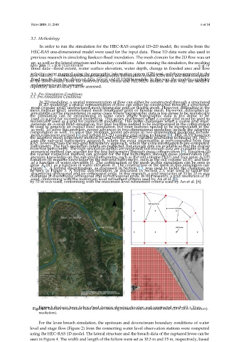
as a function of water elevation H. The construction of the mesh in this simulation can be seen in
areas ( ) as a function of water elevation . The construction of the mesh in this simulation can

Figure 3. A hybrid discretization, as discussed in Section 2.3, was used to tackle the challenge in
be seen in Figure 3. A hybrid discretization, as discussed in Section 2.3, was used to tackle the
discretizing orthogonal and un-orthogonal grids. In this research, a grid resolution of 33 by 33 m was
challenge in discretizing orthogonal and un-orthogonal grids. In this research, a grid resolution of 33
used, conforming with the maximum level refinement criteria used by An et al. [6].
by 33 m was used, conforming with the maximum level refinement criteria used by An et al. [6].

Figure 3. Baeksan levee failure flood domain showing elevation and constructed mesh (33 × 33 m
Figure 3. Baeksan levee failure flood domain showing elevation and constructed mesh (33 × 33 m resolution).
resolution).

For the levee breach simulation, the upstream and downstream boundary conditions of water
level and stage flow (Figure 2) from the connecting water level observation stations were computed
using the HEC-RAS 1D model. The lateral structure and the breach data of the ruptured levee can be
seen in Figure 4. The width and length of the failure were set as 10.3 m and 15 m, respectively, based
on the survey conducted by the Korea Ministry of Construction and Transportation after the event.
The homogeneous roughness coefficient is set to η = 0.06 according to the cultivated crop/pasture
manning value in [ 30], since the flood area is mostly paddy field and vegetable crops [15].