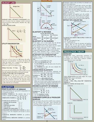
Page 2 - Microeconomics

BUDGET LINE P • Consumer surplus is the area below the demand curve
above the market price.
B • For a given price of a good, there will be some sellers
Budget Line Inelastic who are willing to sell at a lower price. These sellers
Range
Price Level Demand • Therefore, society’s welfare is maximized with the
are receiving extra revenue (producer surplus), since the
price is higher than their willingness to sell.
market clearing price.
Elastic • Both consumers and suppliers gain all available
Range
Q benefits and revenues. Intervention in the market
Quantity (such as taxation, price floors and price ceilings)
A TR lowers society benefits and creates deadweight loss.
• BUDGET LINE or BUDGET CONSTRAINT is the EFFECT OF A SALES TAX
level of income that the consumer needs to allocate Elastic Inelastic New Consumer Surplus
between goods A and B. Equation: Income = (P A × Q A ) Total Revenue Range Range 1
+ (P B × Q B ). Total S
• BUDGET LINE SLOPE Revenue New P* S
A
I Q C
P B I I P Quantity B
Slope = – = – A D
P B P A P B ELASTICITY & REVENUE New
TOTAL REVENUE (TR) Producer Surplus
Price Increase Price Decrease
Elastic TR ↓ TR ↑ New Q*
Unitary Elastic TR unchanged TR unchanged • A SALES TAX SHIFTS THE SUPPLY CURVE TO
I Inelastic TR ↑ TR ↓ THE LEFT.
P A 1. A + B = government revenue
ELASTICITY & TAX BURDEN 2. C = deadweight loss
• If the supply curve is more elastic than the demand
UTILITY MAXIMIZATION curve, consumers carry more of the tax burden. Area C used to be part of consumer and producer
• If the demand curve is more elastic than the supply surplus. With the tax and the new equilibrium
I curve, suppliers carry more of the tax burden. price (P*) and quantity (Q*), neither the consumer,
producer nor the government gets this area.
• If the supply (demand) curve is perfectly elastic,
IV
II consumers (suppliers) carry ALL of the tax burden.
B* • If the supply (demand) curve is perfectly inelastic, PRODUCTION THEORY
suppliers (consumers) carry ALL of the tax burden.
III ELASTICITY AS A DESCRIPTOR ISOQUANT
• ISOQUANT: Curve representing production. It
• If |∈| A > |∈| B , |∈| A is more ELASTIC than |∈| B at
A* given price levels. is similar to an indifference curve, but instead of
• Consumer will not choose I or III because the utility EX: consumption that creates utility, producer combines
inputs (K, L) to create output (Q).
derived is not maximized. Consumer will choose II 1. –0.34 is more ELASTIC than –0.2
where the utility curve is tangent to the budget line. 2. –9.3 is more ELASTIC than –5.6 Capital (K)
Point IV is currently not available. The FLATTER the curve, the more elastic the curve
• Slopes are equal at the tangency point. at every price level. Q = f(K, L)
P MU The STEEPER the curve, the more inelastic the
• Budget Line slope = IC slope A = A curve at every price level.
P B MU B I Q = 300
• Consumers allocate their budget to equate the utility received CROSS-PRICE ELASTICITY Q = 200
from the marginal dollar spent on each good consumed. RESPONSIVENESS OF QUANTITY DEMAND OF II
• UTILITY AND THE LAW OF DEMAND GOOD x TO A CHANGE IN THE PRICE OF GOOD y. Q = 100
y +
P
Qx
Qx −
Py
Relationship: As the price of a good increases, • FORMULA: 2 1 × 2 1 Labor (L)
the utility of the marginal dollar spent on the good RULES: Qx + Qx 1 Py − Py 1 Higher ISOQUANTS mean higher output. On a single
2
2
decreases, since the marginal dollar buys less of the 1. ∈ XY > 0: x, y ARE SUBSTITUTES ISOQUANT, output is unchanged.
good. The consumer reallocates the marginal dollar 2. ∈ XY < 0: x, y ARE COMPLEMENTS EX: Q I = Q II = 100
away from the good, causing quantity demanded to fall In this case, because x and y need to be used together, the SLOPE = – (MP L / MP K ), where MP = MARGINAL
in line with the Law of Demand. behavior is similar to Price Elasticity of Demand for one PRODUCT
good. Note: DO NOT USE ABSOLUTE VALUE! • SPECIAL FORMS OF ISOQUANTS
INCOME ELASTICITY OF DEMAND Capital (K)
ELASTICITY RESPONSIVENESS OF QUANTITY DEMAND TO A
PRICE ELASTICITY OF DEMAND CHANGE IN INCOME.
RESPONSIVENESS OF QUANTITY DEMANDED TO • FORMULA: Q − Q 1 × I + I 1
2
2
A CHANGE IN PRICE. RULES: Q + Q 1 I − I 1
2
2
• SIMPLE FORMULA: The absolute value of % 1. ∈ IE > 0, NORMAL GOOD
change in quantity demanded ÷ % change in price. 2. ∈ IE < 0, INFERIOR GOOD
Q − Q P + P
• MIDPOINTS FORMULA: 2 1 × 2 1 CONSUMER SURPLUS & PRODUCER
Q + Q 1 P − P 1 SURPLUS Labor (L)
2
2
• TYPES OF ELASTICITY (∈): • For a given price of a good, there will be some consumers Perfect Substitutes
1. PERFECTLY ELASTIC |∈| = ∞ who are willing to pay more. These consumers are
2. ELASTIC |∈| > 1 receiving a benefit (consumer surplus), since the price Capital (K)
3. UNITARY ELASTIC |∈| = 1 is lower than their willingness to pay.
4. INELASTIC |∈| < 1 P
5. PERFECTLY INELASTIC |∈| = 0 Consumer
• STRAIGHT LINE DEMAND CURVES are elastic Surplus (CS)
at prices above the midpoint and inelastic at prices
below it. Supply
• VERTICAL DEMAND CURVES are perfectly Market Price
inelastic. Producer Demand
• HORIZONTAL DEMAND CURVES are perfectly Surplus (PS) Labor (L)
elastic. Q Perfect Complements
2