Page 9 - Ranger Demo

cost equipment to deliver in-situ near real-time ocean data. Additional key capabilities for providing ocean data are the use of historical databases, ocean satellite-based measurements and ocean forecast modelling.
The use of underwater glider data is widespread across many defence and academic communities, typically providing a capability for a) the long term gathering of ocean data to support the ocean databases, b) the provision of near real-time data for ocean forecast models to validate their output and to be assimilated into the models as accurate initial conditions and c) to be used by the Royal Navy in the context of a flexible, controllable and recoverable XBT (expendable bathythermograph).
The value in gaining high-quality ocean data for the defence community lies in the ability to understand the propagation of sound in the underwater environment and hence the performance of sonar systems. Propagation of sound underwater is particularly sensitive to spatial gradients in the ocean sound speed structure, which are functions of the temperature and salinity. Some causes of ocean gradients can be due to front, eddies, internal waves, the density-driven ocean circulation patterns, local turbulent microstructure and the passage of weather patterns imparting energy in the ocean. A navy that knows the complexities of the ocean structure can be more effective in its underwater operations, particularly in the use of sonar systems.
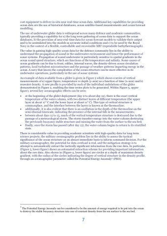
An example of data available from a glider is given in Figure 5 which shows a series of vertical measurements of a) upper figure, temperature vs depth (y-axis) as a function of time (x-axis) and b) seawater density. A new profile is provided by each of the individual undulations of the glider demonstrated in Figure 2, enabling the time series plots to be generated. Within Figure 5, upper figure), several key oceanographic effects can be seen:
at the beginning of the glider deployment (day 0 to about day 12), there is the exact vertical temperature of the water column, with two distinct layers of different temperature (the upper layer at about 17° C and the lower layer at about 11° C). This type of vertical structure is commonplace, and the interface between the layers is known as the thermocline;
additionally, it is also evident that there is an oscillation in the depth of the thermocline on the semi-diurnal timescale, indicating the presence of the internal tide in the measurements;
between about days 12 to 15, much of the vertical temperature structure is destroyed due to the passage of a meteorological storm. The storm transfers energy into the water column destroying the previously buoyancy stable structure and missing the water from the surface to the sea bed;
finally, once the storm has passed (after day 15), the water column begins to return to its stratified state.
There is considerable value in providing academic scientists with high-quality data for long term science projects; the military oceanographic problem lies in the ability to assess the tactical significance of the ocean structure on an almost immediate basis to inform command decision. For the military oceanographer, the potential for data overload is real, and the mitigation strategy is to attempt to automatically extract the tactically significant information from the raw data. In particular, (Figure 5, lower figure) shows an automated extraction scheme for providing important information about the raw data. Also shown in (Figure 5, lower figure) are circles at a depth of maximum density gradient, with the radius of the circles indicating the degree of vertical structure in the density profile, through an oceanographic parameter called the Potential Energy Anomaly3 (PEO).
3 The Potential Energy Anomaly can be considered to be the amount of energy required to be put into the ocean to destroy the stable buoyancy structure into one of constant density from the sea surface to the sea bed.
7