Page 35 - Finanancial Management_Feb_Apr23

Using the UNIQUE function to count unique items in a list

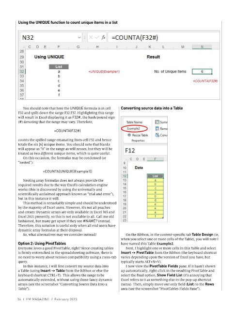
You should note that here the UNIQUE formula is in cell Converting source data into a Table
F32 and spills down the range F32:F37. Highlighting this range
will result in Excel displaying it as F32#, the hash/pound sign
(#) denoting that the range may vary. Therefore,

=COUNTA(F32#)

counts the spilled range emanating from cell F32 and hence
totals the six [6] unique items. You should note that blanks
will appear as “0” in the range as will zeroes, but they will be
treated as two different unique items, which is quite useful.
On this occasion, the formulas may be condensed (or
“nested”):
=COUNTA(UNIQUE(Example1))

Nesting array formulas does not always provide the
required results due to the way Excel’s calculation engine
works (this is discovered by using the universally and
scientifically acclaimed approach known as “trial and error”),
but in this instance it will.
This method is remarkably simple and should be understood
by the majority of Excel users. However, it’s not all peaches
and cream: Dynamic arrays are only available in Excel 365 and
Excel 2021 presently, so this is not available to all. Call me old
fashioned, but many get upset if they see #NAME? instead.
Therefore, this solution is useful only when all end users have
dynamic array formulas at their disposal.
So, what alternatives may we consider instead? On the Ribbon, in the context-specific tab Table Design (ie,
when you select one or more cells of the Table), you will note I
Option 2: Using PivotTables have named this Table Example2.
Everyone loves a good PivotTable, right? Since creating tables Next, I highlight one or more cells in this Table and select
is firmly entrenched in the spreadsheeting software, there is Insert -> PivotTable from the Ribbon (the keyboard shortcut
no need to worry about version compatibility using a cross-tab varies depending upon the version of Excel you have, but
query. typically starts ALT+N+V).
In this instance, I will first convert my source data into I now view the PivotTable Fields pane. If it hasn’t shown
a Table (using Insert -> Table from the Ribbon or else the up automatically, right-click in the resulting PivotTable and
keyboard shortcut CTRL+T). This allows the range to be select the final option, Show Field List (it’s annoying that
automatically extended, without using those fancy dynamic Excel refers to it as something else in the pop-up shortcut
arrays (see the screenshot “Converting Source Data Into a menu). Then, simply move our only field (List) to the Rows
Table”). area (see the screenshot “PivotTables Fields Pane”).

34 I FM MAGAZINE I February 2023