Page 115 - Understanding Machine Learning

9.3 Logistic Regression 97

9.2.2 Linear Regression for Polynomial Regression Tasks
Some learning tasks call for nonlinear predictors, such as polynomial predictors.
Take, for instance, a one dimensional polynomial function of degree n,that is,

2
p(x) = a 0 + a 1 x + a 2 x + ··· + a n x n

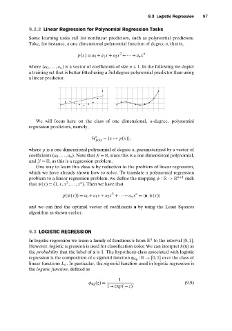
where (a 0 ,...,a n ) is a vector of coefficients of size n + 1. In the following we depict
a training set that is better fitted using a 3rd degree polynomial predictor than using
a linear predictor.

We will focus here on the class of one dimensional, n-degree, polynomial
regression predictors, namely,

n
H poly ={x → p(x)},
where p is a one dimensional polynomial of degree n, parameterized by a vector of
coefficients (a 0 ,...,a n ). Note that X = R, since this is a one dimensional polynomial,
and Y = R, as this is a regression problem.
One way to learn this class is by reduction to the problem of linear regression,
which we have already shown how to solve. To translate a polynomial regression
problem to a linear regression problem, we define the mapping ψ : R → R n+1 such
n
2
that ψ(x) = (1,x,x ,...,x ). Then we have that
2 n
p(ψ(x)) = a 0 + a 1 x + a 2 x + ··· + a n x = a,ψ(x)

and we can find the optimal vector of coefficients a by using the Least Squares
algorithm as shown earlier.

9.3 LOGISTIC REGRESSION

d
In logistic regression we learn a family of functions h from R to the interval [0,1].
However, logistic regression is used for classification tasks: We can interpret h(x)as
the probability that the label of x is 1. The hypothesis class associated with logistic
regression is the composition of a sigmoid function φ sig : R → [0,1] over the class of
linear functions L d . In particular, the sigmoid function used in logistic regression is
the logistic function, defined as

1
φ sig (z) = . (9.9)
1 + exp( − z)