Page 116 - Understanding Machine Learning

Linear Predictors
98

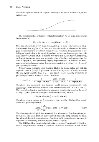
The name “sigmoid” means “S-shaped,” referring to the plot of this function, shown
in the figure:

The hypothesis class is therefore (where for simplicity we are using homogenous
linear functions):
d
H sig = φ sig ◦ L d ={x → φ sig ( w,x ): w ∈ R }.
Note that when w,x is very large then φ sig ( w,x ) is close to 1, whereas if w,x
is very small then φ sig ( w,x ) is close to 0. Recall that the prediction of the halfs-
pace corresponding to a vector w is sign( w,x ). Therefore, the predictions of the
halfspace hypothesis and the logistic hypothesis are very similar whenever | w,x | is
1
large. However, when | w,x | is close to 0 we have that φ sig ( w,x ) ≈ . Intuitively,
2
the logistic hypothesis is not sure about the value of the label so it guesses that the
label is sign( w,x ) with probability slightly larger than 50%. In contrast, the halfs-
pace hypothesis always outputs a deterministic prediction of either 1 or −1, even if
| w,x | is very close to 0.
Next, we need to specify a loss function. That is, we should define how bad it is
to predict some h w (x) ∈ [0,1] given that the true label is y ∈{±1}. Clearly, we would
like that h w (x) would be large if y = 1and that 1 − h w (x) (i.e., the probability of
predicting −1) would be large if y =−1. Note that

1 exp( −w,x ) 1
1 − h w(x) = 1 − = = .
1 + exp( −w,x ) 1 + exp( −w,x ) 1 + exp( w,x )
Therefore, any reasonable loss function would increase monotonically with
1
1+exp(y w,x ) , or equivalently, would increase monotonically with 1+exp(− y w,x ).
The logistic loss function used in logistic regression penalizes h w based on the log of
1 + exp( − y w,x ) (recall that log is a monotonic function). That is,

(h w ,(x, y)) = log 1 + exp( − y w,x ) .
Therefore, given a training set S = (x 1 , y 1 ),...,(x m , y m ), the ERM problem associ-
ated with logistic regression is
m
1
argmin log 1 + exp( − y i w,x i ) . (9.10)
w∈R d m i=1
The advantage of the logistic loss function is that it is a convex function with respect
to w; hence the ERM problem can be solved efficiently using standard methods.
We will study how to learn with convex functions, and in particular specify a simple
algorithm for minimizing convex functions, in later chapters.
The ERM problem associated with logistic regression (Equation (9.10)) is iden-
tical to the problem of finding a Maximum Likelihood Estimator, a well-known