Page 123 - Understanding Machine Learning

10.2 AdaBoost 105

Therefore, we can calculate the objective at θ in a constant time, given the objective
at the previous threshold, θ. It follows that after a preprocessing step in which we
sort the examples with respect to each coordinate, the minimization problem can be
performed in time O(dm). This yields the following pseudocode.

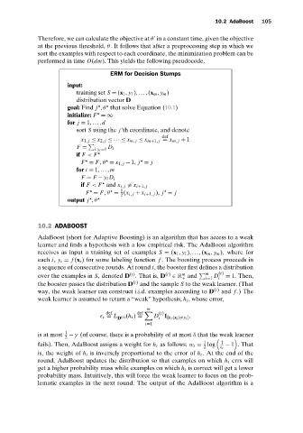
ERM for Decision Stumps
input:
training set S = (x 1 , y 1 ),...,(x m , y m )
distribution vector D

goal: Find j ,θ that solve Equation (10.1)

initialize: F =∞
for j = 1,...,d
sort S using the j’th coordinate, and denote
def
x 1, j ≤ x 2, j ≤ ··· ≤ x m, j ≤ x m+1, j = x m, j + 1

F = D i
i:y i =1
if F < F

F = F, θ = x 1, j − 1, j = j
for i = 1,...,m
F = F − y i D i

if F < F and x i, j = x i+1, j
1

F = F, θ = (x i, j + x i+1, j ), j = j
2

output j ,θ
10.2 ADABOOST
AdaBoost (short for Adaptive Boosting) is an algorithm that has access to a weak
learner and finds a hypothesis with a low empirical risk. The AdaBoost algorithm
receives as input a training set of examples S = (x 1 , y 1 ),...,(x m , y m ), where for
each i, y i = f (x i ) for some labeling function f . The boosting process proceeds in
a sequence of consecutive rounds. At round t, the booster first defines a distribution
(t)
m
over the examples in S, denoted D .That is, D (t) ∈ R and m D (t) = 1. Then,
+ i=1 i
the booster passes the distribution D (t) and the sample S to the weak learner. (That
way, the weak learner can construct i.i.d. examples according to D (t) and f .) The
weak learner is assumed to return a “weak” hypothesis, h t , whose error,
m
def def (t)

t = L (t)(h t ) = D 1 [h t (x i ) =y i ] ,
D i
i=1
is at most 1 − γ (of course, there is a probability of at most δ that the weak learner
2

1
fails). Then, AdaBoost assigns a weight for h t as follows: w t = log 1 − 1 .That
2
t
is, the weight of h t is inversely proportional to the error of h t . Atthe end ofthe
round, AdaBoost updates the distribution so that examples on which h t errs will
get a higher probability mass while examples on which h t is correct will get a lower
probability mass. Intuitively, this will force the weak learner to focus on the prob-
lematic examples in the next round. The output of the AdaBoost algorithm is a