Page 125 - Understanding Machine Learning

10.2 AdaBoost 107

Hence,
m −y i f t+1 ( x i )

Z t+1 i=1 e
=
m

Z t −y j f t ( x j )

e
j=1
m −y i f t ( x i ) −y i w t+1 h t+1 ( x i )

i=1 e e
=

m

e −y j f t ( x j )

j=1
m
( t+1) −y i w t+1 h t+1 ( x i )

= D e
i
i=1
( t+1) ( t+1)
= e −w t+1 D i + e w t+1 D i

i: y i h t+1 ( x i )=1 i: y i h t+1 ( x i )=−1

= e −w t+1 (1 −
t+1 ) + e w t+1
t+1
1
(1 −
t+1 ) +
= 1/
t+1 − 1
t+1
1/
t+1 − 1
*

t+1 1 −
t+1
= (1 −
t+1 ) +
t+1
1 −
t+1
t+1

= 2
t+1 (1 −
t+1 ).
1

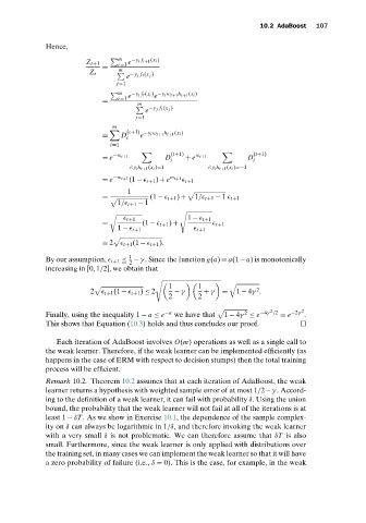
By our assumption,
t+1 ≤ −γ . Since the function g(a) = a(1−a) is monotonically
2
increasing in [0,1/2], we obtain that
*

1 1
2
2
t+1 (1 −
t+1 ) ≤ 2 − γ + γ = 1 − 4γ .
2 2
2 2
2

Finally, using the inequality 1 − a ≤ e −a we have that 1 − 4γ ≤ e −4γ /2 = e −2γ .

This shows that Equation (10.3) holds and thus concludes our proof.
Each iteration of AdaBoost involves O(m) operations as well as a single call to
the weak learner. Therefore, if the weak learner can be implemented efficiently (as
happens in the case of ERM with respect to decision stumps) then the total training
process will be efficient.
Remark 10.2. Theorem 10.2 assumes that at each iteration of AdaBoost, the weak
learner returns a hypothesis with weighted sample error of at most 1/2−γ . Accord-
ing to the definition of a weak learner, it can fail with probability δ. Using the union
bound, the probability that the weak learner will not fail at all of the iterations is at
least 1 − δT . As we show in Exercise 10.1, the dependence of the sample complex-

ity on δ can always be logarithmic in 1/δ, and therefore invoking the weak learner
with a very small δ is not problematic. We can therefore assume that δT is also
small. Furthermore, since the weak learner is only applied with distributions over
the training set, in many cases we can implement the weak learner so that it will have
a zero probability of failure (i.e., δ = 0). This is the case, for example, in the weak