Page 170 - Understanding Machine Learning

Stochastic Gradient Descent
152

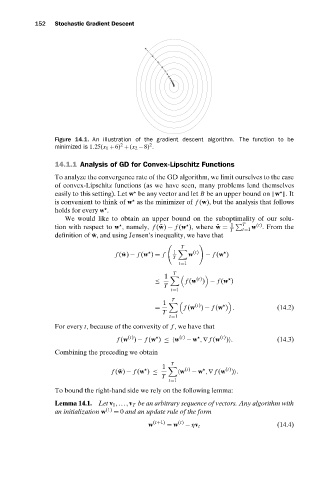
Figure 14.1. An illustration of the gradient descent algorithm. The function to be
2
2
minimized is 1.25(x 1 + 6) + (x 2 − 8) .
14.1.1 Analysis of GD for Convex-Lipschitz Functions

To analyze the convergence rate of the GD algorithm, we limit ourselves to the case
of convex-Lipschitz functions (as we have seen, many problems lend themselves

easily to this setting). Let w be any vector and let B be an upper bound on w .It

is convenient to think of w as the minimizer of f (w), but the analysis that follows

holds for every w .
We would like to obtain an upper bound on the suboptimality of our solu-
1 T (t)
tion with respect to w , namely, f ( ¯ w) − f (w ), where ¯ w = w .From the
T t=1
definition of ¯ w, and using Jensen’s inequality, we have that

T

f ( ¯ w) − f (w ) = f 1 w (t) − f (w )
T
t=1
1 (t)
T
≤ f (w ) − f (w )
T
t=1
1 (t)
T
= f (w ) − f (w ) . (14.2)
T
t=1
For every t, because of the convexity of f , we have that

(t)
(t)

f (w ) − f (w ) ≤ø w (t) − w ,∇ f (w ) . (14.3)
Combining the preceding we obtain
T
1
(t) (t)
f ( ¯ w) − f (w ) ≤ w − w ,∇ f (w ) .
T
t=1
To bound the right-hand side we rely on the following lemma:
Lemma 14.1. Let v 1 ,...,v T be an arbitrary sequence of vectors. Any algorithm with
an initialization w (1) = 0 and an update rule of the form
w (t+1) = w (t) − ηv t (14.4)