Page 175 - Understanding Machine Learning

14.3 Stochastic Gradient Descent (SGD) 157

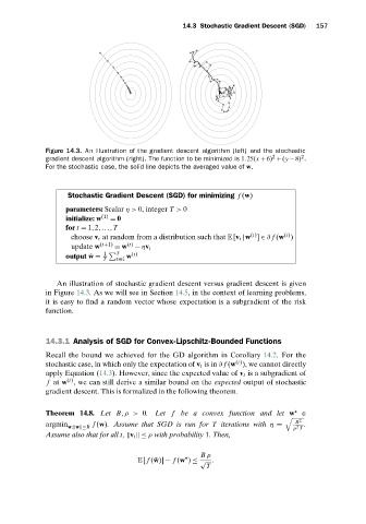
Figure 14.3. An illustration of the gradient descent algorithm (left) and the stochastic
2
2
gradient descent algorithm (right). The function to be minimized is 1.25(x +6) +(y −8) .
For the stochastic case, the solid line depicts the averaged value of w.

Stochastic Gradient Descent (SGD) for minimizing f (w)
parameters: Scalar η> 0, integer T > 0
initialize: w (1) = 0
for t = 1,2,...,T
(t)
(t)
choose v t at random from a distribution such that E[v t |w ] ∈ ∂ f (w )
update w (t+1) = w (t) − ηv t
1 T (t)
output ¯ w = w
T t=1
An illustration of stochastic gradient descent versus gradient descent is given
in Figure 14.3. As wewill seeinSection 14.5, in the context of learning problems,
it is easy to find a random vector whose expectation is a subgradient of the risk
function.

14.3.1 Analysis of SGD for Convex-Lipschitz-Bounded Functions
Recall the bound we achieved for the GD algorithm in Corollary 14.2.For the
(t)
stochastic case, in which only the expectation of v t is in ∂ f (w ), we cannot directly
apply Equation (14.3). However, since the expected value of v t is a subgradient of
(t)
f at w , we can still derive a similar bound on the expected output of stochastic
gradient descent. This is formalized in the following theorem.

Theorem 14.8. Let B,ρ > 0.Let f be a convex function and let w ∈
2
argmin f (w). Assume that SGD is run for T iterations with η = B .
w: w ≤B ρ T
2
Assume also that for all t, v t ≤ ρ with probability 1. Then,
B ρ

E[ f ( ¯ w)] − f (w ) ≤ √ .
T