Page 179 - Understanding Machine Learning

14.4 Variants 161

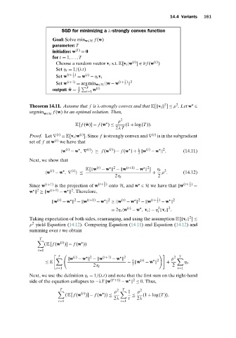
SGD for minimizing a λ-strongly convex function
Goal: Solve min w∈H f (w)
parameter: T
initialize: w (1) = 0
for t = 1,...,T
(t)
(t)
Choose a random vector v t s.t. E[v t |w ] ∈ ∂ f (w )
Set η t = 1/(λt)
1
Set w (t+ ) (t) − η t v t
2 = w
1
Set w (t+1) = argmin w∈H w − w (t+ ) 2
2
1 T (t)
output: ¯ w = w
T t=1
2 2
Theorem 14.11. Assume that f is λ-strongly convex and that E[ v t ] ≤ ρ .Let w ∈
argmin f (w) be an optimal solution. Then,
w∈H
ρ 2

E[ f ( ¯ w)] − f (w ) ≤ (1 + log(T )).
2λT
(t) (t) (t)
Proof. Let ∇ = E[v t |w ]. Since f is strongly convex and ∇ is in the subgradient
set of f at w (t) we have that
(t)
2
(t)

λ

w (t) − w , ∇ ≥ f (w ) − f (w ) + w (t) − w . (14.11)
2
Next, we show that
2
2
E[ w (t) − w −⊂w (t+1) − w ] η t 2
(t)
(t)

w − w , ∇ ≤ + ρ . (14.12)
2η t 2
1
1
2 onto H,and w ∈ H we have that w
Since w (t+1) is the projection of w (t+ ) (t+ )
2 −
2
2
w ≥√w (t+1) − w . Therefore,
1
2
2
2
w (t) − w −⊂w (t+1) − w ≥√w (t) − w −⊂w (t+ ) 2
2 − w
2
2

= 2η t w (t) − w , v t − η v t .
t
2
Taking expectation of both sides, rearranging, and using the assumption E[ v t ] ≤
2
ρ yield Equation (14.12). Comparing Equation (14.11) and Equation (14.12)and
summing over t we obtain
T
(t)
(E[ f (w )] − f (w ))
t=1

T (t) 2 (t+1) 2 T
w − w −⊂w − w ρ 2
2
λ
≤ E − w (t) − w + η t .
2
2η t 2
t=1 t=1
Next, we use the definition η t = 1/(λt) and note that the first sum on the right-hand
2
side of the equation collapses to −λT w (T +1) − w ≤ 0. Thus,
T T 2
ρ 2 1 ρ
(t)
(E[ f (w )] − f (w )) ≤ ≤ (1 + log(T )).
2λ t 2λ
t=1 t=1