Page 181 - Understanding Machine Learning

14.5 Learning with SGD 163

(t)
(t)
It follows that E[v t |w ] is a subgradient of L D (w)at w .
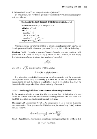
To summarize, the stochastic gradient descent framework for minimizing the
risk is as follows.

Stochastic Gradient Descent (SGD) for minimizing L D (w)
parameters: Scalar η> 0, integer T > 0
initialize: w (1) = 0
for t = 1,2,...,T
sample z ∼ D
(t)
pick v t ∈ ∂Ø (w ,z)
update w (t+1) = w (t) − ηv t
1 T (t)
output ¯ w = w
T t=1
We shall now use our analysis of SGD to obtain a sample complexity analysis for
learning convex-Lipschitz-bounded problems. Theorem 14.8 yields the following:
Corollary 14.12. Consider a convex-Lipschitz-bounded learning problem with
parameters ρ, B. Then, for every
> 0, if we run the SGD method for minimizing
L D (w) with a number of iterations (i.e., number of examples)

2 2
B ρ
T ≥

2

B 2
and with η = 2 , then the output of SGD satisfies
ρ T
E[L D ( ¯ w)] ≤ min L D (w) +
.
w∈H
It is interesting to note that the required sample complexity is of the same order
of magnitude as the sample complexity guarantee we derived for regularized loss
minimization. In fact, the sample complexity of SGD is even better than what we
have derived for regularized loss minimization by a factor of 8.

14.5.2 Analyzing SGD for Convex-Smooth Learning Problems
In the previous chapter we saw that the regularized loss minimization rule also
learns the class of convex-smooth-bounded learning problems. We now show that
the SGD algorithm can be also used for such problems.
Theorem 14.13. Assume that for all z, the loss function (·,z) is convex, β-smooth,
and nonnegative. Then, if we run the SGD algorithm for minimizing L D (w) we have

that for every w ,

2
1 w
E[L D ( ¯ w)] ≤ L D (w ) + .
1 − ηβ 2η T
Proof. Recall that if a function is β-smooth and nonnegative then it is self-bounded:
2
∇ f (w) ≤ 2β f (w).