Page 182 - Understanding Machine Learning

Stochastic Gradient Descent
164

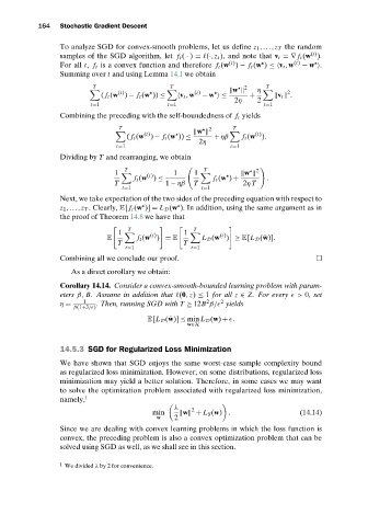
To analyze SGD for convex-smooth problems, let us define z 1 ,...,z T the random
(t)
samples of the SGD algorithm, let f t ( · ) = (·,z t ), and note that v t =∇ f t (w ).

(t)
For all t, f t is a convex function and therefore f t (w ) − f t (w ) ≤ø v t ,w (t) − w .
Summing over t and using Lemma 14.1 we obtain
T T 2 T
w η
(t) (t) 2
( f t (w ) − f t (w )) ≤ v t ,w − w ≤ + v t .
2η 2
t=1 t=1 t=1
Combining the preceding with the self-boundedness of f t yields
T 2 T
w
(t) (t)
( f t (w ) − f t (w )) ≤ + ηβ f t (w ).
2η
t=1 t=1
Dividing by T and rearranging, we obtain
T T 2
1 (t) 1 1 w
f t (w ) ≤ f t (w ) + .
T 1 − ηβ T 2η T
t=1 t=1
Next, we take expectation of the two sides of the preceding equation with respect to

z 1 ,...,z T . Clearly, E[ f t (w )] = L D (w ). In addition, using the same argument as in
the proof of Theorem 14.8 we have that
T T
1 (t) 1 (t)
E f t (w ) = E L D (w ) ≥ E[L D ( ¯ w)].
T T
t=1 t=1
Combining all we conclude our proof.
As a direct corollary we obtain:
Corollary 14.14. Consider a convex-smooth-bounded learning problem with param-
eters β, B. Assume in addition that (0, z) ≤ 1 for all z ∈ Z. For every
> 0,set
1 2 2
η = . Then, running SGD with T ≥ 12B β/
yields
β(1+3/
)
E[L D ( ¯ w)] ≤ min L D (w) +
.
w∈H

14.5.3 SGD for Regularized Loss Minimization

We have shown that SGD enjoys the same worst-case sample complexity bound
as regularized loss minimization. However, on some distributions, regularized loss
minimization may yield a better solution. Therefore, in some cases we may want
to solve the optimization problem associated with regularized loss minimization,
namely, 1

λ 2
min w + L S (w) . (14.14)
w 2
Since we are dealing with convex learning problems in which the loss function is
convex, the preceding problem is also a convex optimization problem that can be
solved using SGD as well, as we shall see in this section.

1 We divided λ by 2 for convenience.