Page 257 - Understanding Machine Learning

20.6 SGD and Backpropagation 239

obtain that the loss, as a function of W t−1 , can be written as
g t (W t−1 ) = t (o t ) = t (σ(a t )) = t (σ(W t−1 o t−1 )).
It would be convenient to rewrite this as follows. Let w t−1 ∈ R k t−1 k t be the column
vector obtained by concatenating the rows of W t−1 and then taking the transpose of
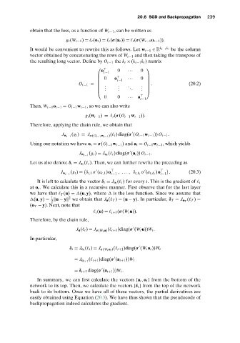
the resulting long vector. Define by O t−1 the k t × (k t−1 k t )matrix
 
o
0 ··· 0
t−1

 0 o
··· 0 

t−1
 
O t−1 =  . . . . . (20.2)
 . . .
 . . . . 
. 
0 0 ··· o
t−1
Then, W t−1 o t−1 = O t−1 w t−1 , so we can also write
g t (w t−1 ) = t (σ(O t−1 w t−1 )).
Therefore, applying the chain rule, we obtain that
(g t ) = J σ(O t−1 w t−1 ) ( t )diag(σ (O t−1 w t−1 )) O t−1 .

J w t−1
Using our notation we have o t = σ(O t−1 w t−1 )and a t = O t−1 w t−1 , which yields
( t )diag(σ (a t )) O t−1 .

J w t−1 (g t ) = J o t
( t ). Then, we can further rewrite the preceding as
Let us also denote δ t = J o t

(g t ) = δ t,1 σ (a t,1 )o
)o
. (20.3)
J w t−1 t−1 , ... , δ t,k t σ (a t,k t t−1
It is left to calculate the vector δ t = J o t ( t ) for every t. This is the gradient of t
at o t . We calculate this in a recursive manner. First observe that for the last layer
we have that T (u) = (u,y), where is the loss function. Since we assume that
1 2
2
(u,y) = u − y we obtain that J u ( T ) = (u − y). In particular, δ T = J o T ( T ) =
(o T − y). Next, note that
t (u) = t+1 (σ(W t u)).
Therefore, by the chain rule,

J u ( t ) = J σ(W t u) ( t+1 )diag(σ (W t u))W t .

In particular,

δ t = J o t ( t ) = J σ(W t o t ) ( t+1 )diag(σ (W t o t ))W t

( t+1 )diag(σ (a t+1 ))W t
= J o t+1
= δ t+1 diag(σ (a t+1 ))W t .

In summary, we can first calculate the vectors {a t ,o t } from the bottom of the
network to its top. Then, we calculate the vectors {δ t } from the top of the network
back to its bottom. Once we have all of these vectors, the partial derivatives are
easily obtained using Equation (20.3). We have thus shown that the pseudocode of
backpropagation indeed calculates the gradient.