Page 265 - Understanding Machine Learning

21. 1 Online C lassification in the Realizable Case 247

In PAC learning, we identified ERM as a good learning algorithm, in the sense
that if H is learnable then it is learnable by the rule ERM H . A natural learning rule

for online learning is to use (at any online round) any ERM hypothesis, namely, any
hypothesis which is consistent with all past examples.

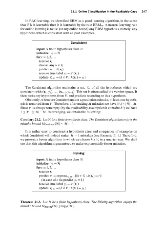
Consistent

input: A finite hypothesis class H
initialize: V 1 = H

for t = 1,2,...
receive x t

choose any h ∈ V t

predict p t = h(x t )

receive true label y t = h (x t )

update V t+1 = {h ∈ V t : h(x t ) = y t }

The Consistent algorithm maintains a set, V t , of all the hypotheses which are

consistent with (x 1 , y 1 ),...,(x t−1 , y t−1 ). This set is often called the version space. It

then picks any hypothesis from V t and predicts according to this hypothesis.

Obviously, whenever Consistent makes a prediction mistake, at least one hypoth-

esis is removed from V t . Therefore, after making M mistakes we have |V t |≤ |H|− M.

Since V t is always nonempty (by the realizability assumption it contains h ) we have

1 ≤ |V t |≤ |H|− M. Rearranging, we obtain the following:

Corollary 21.2. Let H be a finite hypothesis class. The Consistent algorithm enjoys the

mistake bound M Consistent (H) ≤|H|− 1.
It is rather easy to construct a hypothesis class and a sequence of examples on

which Consistent will indeed make |H|− 1 mistakes (see Exercise 21.1.) Therefore,

we present a better algorithm in which we choose h ∈ V t in a smarter way. We shall
see that this algorithm is guaranteed to make exponentially fewer mistakes.
Halving
input: A finite hypothesis class H
initialize: V 1 = H
for t = 1,2,...
receive x t
predict p t = argmax |{h ∈ V t : h(x t ) = r}|
r∈{0,1}
(incaseofa tiepredict p t = 1)

receive true label y t = h (x t )
update V t+1 ={h ∈ V t : h(x t ) = y t }
Theorem 21.3. Let H be a finite hypothesis class. The Halving algorithm enjoys the
mistake bound M Halving (H) ≤ log (|H|).
2