Page 86 - Understanding Machine Learning

Nonuniform Learnability
68

of the error that stems from estimation error and therefore know how much of the
error is attributed to approximation error. If the approximation error is large, we
know that we should use a different hypothesis class. Similarly, if a nonuniform
algorithm fails, we can consider a different weighting function over (subsets of)
hypotheses. However, when a consistent algorithm fails, we have no idea whether
this is because of the estimation error or the approximation error. Furthermore,
even if we are sure we have a problem with the estimation error term, we do not
know how many more examples are needed to make the estimation error small.

How to Learn? How to Express Prior Knowledge?
Maybe the most useful aspect of the theory of learning is in providing an answer to
the question of “how to learn.” The definition of PAC learning yields the limitation
of learning (via the No-Free-Lunch theorem) and the necessity of prior knowledge.
It gives us a crisp way to encode prior knowledge by choosing a hypothesis class,
and once this choice is made, we have a generic learning rule – ERM. The definition
of nonuniform learnability also yields a crisp way to encode prior knowledge by
specifying weights over (subsets of) hypotheses of H. Once this choice is made, we
again have a generic learning rule – SRM. The SRM rule is also advantageous in
model selection tasks, where prior knowledge is partial. We elaborate on model
selection in Chapter 11 and here we give a brief example.
Consider the problem of fitting a one dimensional polynomial to data; namely,
our goal is to learn a function, h : R → R, and as prior knowledge we consider the
hypothesis class of polynomials. However, we might be uncertain regarding which
degree d would give the best results for our data set: A small degree might not fit
the data well (i.e., it will have a large approximation error), whereas a high degree
might lead to overfitting (i.e., it will have a large estimation error). In the follow-
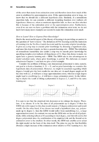
ing we depict the result of fitting a polynomial of degrees 2, 3, and 10 to the same
training set.

Degree 2 Degree 3 Degree 10

It is easy to see that the empirical risk decreases as we enlarge the degree. There-
fore, if we choose H to be the class of all polynomials up to degree 10 then the
ERM rule with respect to this class would output a 10 degree polynomial and would
overfit. On the other hand, if we choose too small a hypothesis class, say, polyno-
mials up to degree 2, then the ERM would suffer from underfitting (i.e., a large
approximation error). In contrast, we can use the SRM rule on the set of all polyno-
mials, while ordering subsets of H according to their degree, and this will yield a 3rd
degree polynomial since the combination of its empirical risk and the bound on its
estimation error is the smallest. In other words, the SRM rule enables us to select
the right model on the basis of the data itself. The price we pay for this flexibility
(besides a slight increase of the estimation error relative to PAC learning w.r.t. the