Page 45 - Data Science Algorithms in a Week

30 Edwin Cortes, Luis Rabelo and Gene Lee

Zhang et al. (2014) stated that learning in an RBM is accomplished by using training
data and “adjusting the RBM parameters such that the probability distribution represented
by the RBM fits the training data as well as possible.” RBMs are energy-based models.
As such, a scalar energy is associated to each variable configuration. Per Bengio (2009),
learning from data corresponds to performing a modification of the energy function until
its shape represents the properties needed. This energy function has different forms
depending on the type of RBM it represents. Binary RBMs, also known as Bernoulli
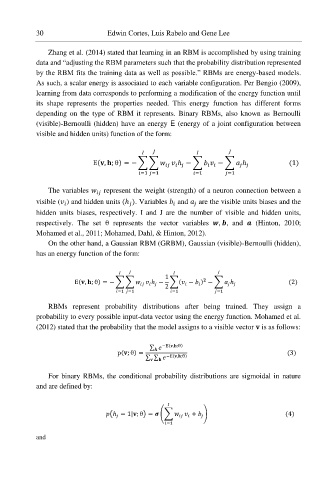
(visible)-Bernoulli (hidden) have an energy E (energy of a joint configuration between
visible and hidden units) function of the form:

E( , ; θ) = − ∑ ∑ ℎ − ∑ − ∑ ℎ (1)

=1 =1 =1 =1

The variables represent the weight (strength) of a neuron connection between a

visible ( ) and hidden units (ℎ ). Variables and are the visible units biases and the

hidden units biases, respectively. I and J are the number of visible and hidden units,
respectively. The set θ represents the vector variables , , and (Hinton, 2010;
Mohamed et al., 2011; Mohamed, Dahl, & Hinton, 2012).
On the other hand, a Gaussian RBM (GRBM), Gaussian (visible)-Bernoulli (hidden),
has an energy function of the form:

1

E( , ; θ) = − ∑ ∑ ℎ − ∑( − ) − ∑ ℎ (2)

2
=1 =1 =1 =1

RBMs represent probability distributions after being trained. They assign a
probability to every possible input-data vector using the energy function. Mohamed et al.
(2012) stated that the probability that the model assigns to a visible vector is as follows:

∑ −E( , ;θ)
p( ; θ) = (3)
∑ ∑ −E( , ;θ)

For binary RBMs, the conditional probability distributions are sigmoidal in nature
and are defined by:

(ℎ = 1| ; θ) = (∑ + ) (4)

=1

and