Page 46 - Data Science Algorithms in a Week

Using Deep Learning to Configure Parallel Distributed Discrete-Event Simulators 31

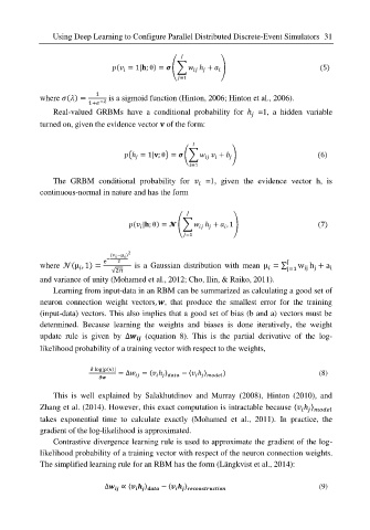
( = 1| ; θ) = (∑ ℎ + ) (5)

=1

where ( ) = 1 is a sigmoid function (Hinton, 2006; Hinton et al., 2006).
1+ −
Real-valued GRBMs have a conditional probability for ℎ =1, a hidden variable

turned on, given the evidence vector of the form:

(ℎ = 1| ; θ) = (∑ + ) (6)

=1

The GRBM conditional probability for =1, given the evidence vector h, is

continuous-normal in nature and has the form

( | ; θ) = (∑ ℎ + , 1) (7)

=1

(v −μ ) 2
i

−
2
where (μ , 1) = e √2π is a Gaussian distribution with mean μ = ∑ J j=1 w h + a
ij
i

j

and variance of unity (Mohamed et al., 2012; Cho, Ilin, & Raiko, 2011).
Learning from input-data in an RBM can be summarized as calculating a good set of
neuron connection weight vectors, , that produce the smallest error for the training
(input-data) vectors. This also implies that a good set of bias (b and a) vectors must be
determined. Because learning the weights and biases is done iteratively, the weight
update rule is given by ∆ (equation 8). This is the partial derivative of the log-

likelihood probability of a training vector with respect to the weights,

∂ log [p( )]
= ∆ = 〈 ℎ 〉 − 〈 ℎ 〉 ) (8)

This is well explained by Salakhutdinov and Murray (2008), Hinton (2010), and
Zhang et al. (2014). However, this exact computation is intractable because 〈 ℎ 〉

takes exponential time to calculate exactly (Mohamed et al., 2011). In practice, the
gradient of the log-likelihood is approximated.
Contrastive divergence learning rule is used to approximate the gradient of the log-
likelihood probability of a training vector with respect of the neuron connection weights.
The simplified learning rule for an RBM has the form (Längkvist et al., 2014):

∆ ∝ 〈 〉 − 〈 〉 (9)