Page 35 - Servo Motors and Industrial Control Theory

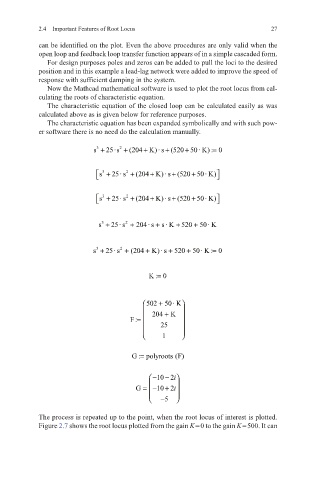
2.4 Important Features of Root Locus 27

can be identified on the plot. Even the above procedures are only valid when the
open loop and feedback loop transfer function appears of in a simple cascaded form.
For design purposes poles and zeros can be added to pull the loci to the desired
position and in this example a lead-lag network were added to improve the speed of
response with sufficient damping in the system.
Now the Mathcad mathematical software is used to plot the root locus from cal-
culating the roots of characteristic equation.
The characteristic equation of the closed loop can be calculated easily as was
calculated above as is given below for reference purposes.
The characteristic equation has been expanded symbolically and with such pow-
er software there is no need do the calculation manually.

s + 25·s + (204 K) · s (520 50· K) : 0+ + + =
2
3
+
+
+
3
2
 s  + 25· s + (204 K) · s (520 50· K) 
+
+
+
2
3
 s  + 25· s + (204 K) · s (520 50· K) 
s + 25· s + 204· s + s · K + 520 + 50· K
2
3
3
2
s + 25· s + (204 + K) · s + 520 + 50· K : 0=
K: 0=

 502 + 50· K
 204 + K 
F:  
=
 25 
  1  

G : polyroots (F)=

 − 10 2i− 

G =− 10 2i+ 
 
 − 5 

The process is repeated up to the point, when the root locus of interest is plotted.
Figure 2.7 shows the root locus plotted from the gain K = 0 to the gain K = 500. It can