Page 85 - Servo Motors and Industrial Control Theory

78 4 Electrical DC Servo Motors

100 % efficient motors. The motor in consideration is separately excited. The trans-
mission mechanism can be idealized by a shaft with stiffness of 1000 Nm/rad. This
is an example for the sake of numerical analysis. For real application, the stiffness
must be calculated from the design configuration of the system.
It is assumed that a gearbox is attached to the motor with input/output speed ra-
tio of N = 10. For most poison control servos, a gearbox must be used to reduce the
speed to an acceptable level. The DC servo motors are available at various output
torque and speed configurations depending on the design of motor. Various motors
must be tried to find the most suitable one. For the purpose of analysis the power
unit is considered an ideal amplifier that converts low-level signal to high voltage
and current output. The properties of various power units will be studied at the end
of this chapter. Selecting a motor can be started by matching the load inertia to the
motor inertia. The rule of thumb is that they should be equal or less than the rotor
inertia. In this calculation, the effect of gearbox which reduces the effect of load
2
inertia by a factor of 1/N must be taken into account. In this example, it is assumed
that the load inertia is 0.078 kg m . The MathCad software is used to study the dy-
2
namic behavior of the system as follows:

K : 1000=
s
R :=0.36
L :=0.88·10 − 3
C : 0.83=
m
J :=7.8·10 − 3 (4.21)
m
J :=78·10 − 3
1
C :=0
1
C := 0
N :=10
K :=100

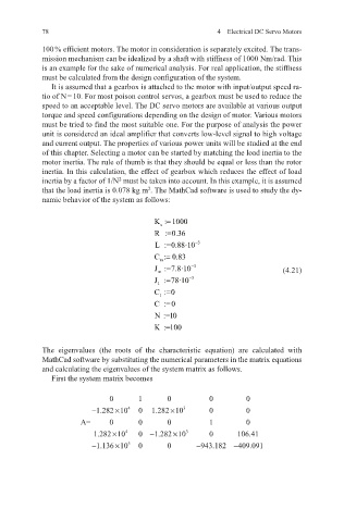
The eigenvalues (the roots of the characteristic equation) are calculated with
MathCad software by substituting the numerical parameters in the matrix equations
and calculating the eigenvalues of the system matrix as follows.
First the system matrix becomes

0 1 0 0 0
−1 282. ×10 4 0 1 282. ×10 3 0 0
A= 0 0 0 1 0
1 282. ×10 4 0 −1 282. ×10 3 0 106..41
− . 1 136 10× 5 0 0 − 943 .182 − 409 .091