Page 86 - Servo Motors and Industrial Control Theory

4.6 DC Servo Motors for Very High Performance Requirements 79

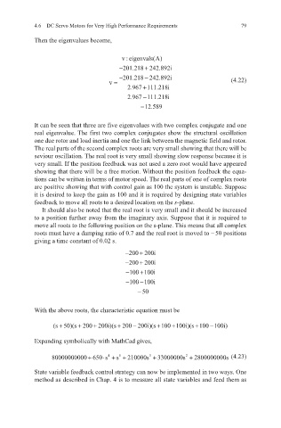
Then the eigenvalues become,

veigenvals A: ( )
−201 .218 + 242 .892 i
−201 .218 − 242 .892 i
v = (4.22)
. 2 967 +1111 218. i
2 967 111 218. − . i
− 12 589.

It can be seen that three are five eigenvalues with two complex conjugate and one
real eigenvalue. The first two complex conjugates show the structural oscillation
one due rotor and load inertia and one the link between the magnetic field and rotor.
The real parts of the second complex roots are very small showing that there will be
seviour oscillation. The real root is very small showing slow response because it is
very small. If the position feedback was not used a zero root would have appeared
showing that there will be a free motion. Without the position feedback the equa-
tions can be written in terms of motor speed. The real parts of one of complex roots
are positive showing that with control gain as 100 the system is unstable. Suppose
it is desired to keep the gain as 100 and it is required by designing state variables
feedback to move all roots to a desired location on the s-plane.
It should also be noted that the real root is very small and it should be increased
to a position further away from the imaginary axis. Suppose that it is required to
move all roots to the following position on the s-plane. This means that all complex
roots must have a damping ratio of 0.7 and the real root is moved to − 50 positions
giving a time constant of 0.02 s.
+
−200 200i
+
−200 200i
−100 +100i
−100 −100i
− 50

With the above roots, the characteristic equation must be
−
+
(s + 50 )(s + 200 200 )( is + 200 200 )( is +100 +100 )( is +100 −100 ) i
Expanding symbolically with MathCad gives,

80000000000 650+ ⋅s 4 + s 5 + 210000 +s 3 33000000 +s 2 2800000000s (4.23)

State variable feedback control strategy can now be implemented in two ways. One
method as described in Chap. 4 is to measure all state variables and feed them as