Page 91 - Servo Motors and Industrial Control Theory

84 4 Electrical DC Servo Motors

2
2
1.5 Output
F1(α) Voltage
1
F2(α)
0.5
Gain
0
0 45 90 135 180
0 α 180

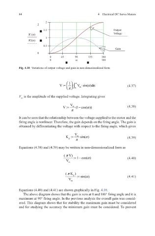
Fig. 4.10 Variations of output voltage and gain in non-dimesionalized form

1
 ∫
α
V :=  · 0 α V ·sin( )dα (4.37)

π
m
V is the amplitude of the supplied voltage. Integrating gives
m

V := V m ·(1 cos( ))α− (4.38)
π
It can be seen that the relationship between the voltage supplied to the motor and the
firing angle is nonlinear. Therefore, the gain depends on the firing angle. The gain is
obtained by differentiating the voltage with respect to the firing angle, which gives
V
K := m ·sin( )α (4.39)
g π

Equations (4.38) and (4.39) may be written in non-dimensionalized form as
( V)π
=−
V : 1 cos( )α (4.40)
m

( K )π
g : sin( )α= (4.41)
V
m

Equations (4.40) and (4.41) are shown graphically in Fig. 4.10.
The above diagram shows that the gain is zero at 0 and 180° firing angle and it is
maximum at 90° firing angle. In the previous analysis the overall gain was consid-
ered. This diagram shows that for stability the maximum gain must be considered
and for studying the accuracy the minimum gain must be considered. To prevent