Page 39 - Microeconomics, Fourth Edition

c01analyzingeconomicproblems.qxd 6/21/10 8:47 AM Page 13

1.2 THREE KEY ANALYTICAL TOOLS 13

Price per pound (dollars) $2.50 Excess Suppl y ( S )

suppl y

$2.00

$1.50
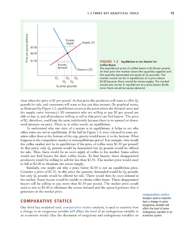
Excess FIGURE 1.2 Equilibrium in the Market for
Coffee Beans
demand The equilibrium price of coffee beans is $2.00 per pound.
Demand ( D )
At that price the market clears (the quantity supplied and
the quantity demanded are equal at Q 3 pounds). The
Q Q Q
1 3 5 market would not be in equilibrium at a price above
Q Q
2 4 $2.00 because there would be excess supply. The market
would also not be in equilibrium at a price below $2.00,
Quantity (pounds)
since there would be excess demand.
clear when the price is $2 per pound. At that price the producers will want to offer Q 3
pounds for sale, and consumers will want to buy just that amount. (In graphical terms,
as illustrated by Figure 1.2, equilibrium occurs at the point where the demand curve and
the supply curve intersect.) All consumers who are willing to pay $2 per pound are
able to buy it, and all producers willing to sell at that price can find buyers. The price
of $2, therefore, could stay the same indefinitely because there is no upward or down-
ward pressure on price. There is, in other words, an equilibrium.
To understand why one state of a system is in equilibrium, it helps to see why
other states are not in equilibrium. If the ball in Figure 1.1, were released at some po-
sition other than at the bottom of the cup, gravity would move it to the bottom. What
happens in the competitive market at nonequilibrium prices? For example, why would
the coffee market not be in equilibrium if the price of coffee were $2.50 per pound?
At that price, only Q 2 pounds would be demanded, but Q 5 pounds would be offered
for sale. Thus, there would be an excess supply of coffee in the market. Some sellers
would not find buyers for their coffee beans. To find buyers, these disappointed
producers would be willing to sell for less than $2.50. The market price would need
to fall to $2.00 to eliminate the excess supply.
Similarly, one might ask why a price below $2.00 is not an equilibrium price.
Consider a price of $1.50. At this price the quantity demanded would be Q 4 pounds,
but only Q 1 pounds would be offered for sale. There would then be excess demand in
the market. Some buyers would be unable to obtain coffee beans. These disappointed
buyers will be willing to pay more than $1.50 per pound. The market price would
need to rise to $2.00 to eliminate the excess demand and the upward pressure that it
generates on the market price.
comparative statics
Analysis used to examine
COMPARATIVE STATICS how a change in some
exogenous variable will
Our third key analytical tool, comparative statics analysis, is used to examine how affect the level of some
a change in an exogenous variable will affect the level of an endogenous variable in endogenous variable in an
an economic model. (See the discussion of exogenous and endogenous variables on economic system.