Page 42 - Microeconomics, Fourth Edition

c01analyzingeconomicproblems.qxd 7/14/10 11:05 AM Page 16

16 CHAPTER 1 ANALYZING ECONOMIC PROBLEMS

S

Price per badge (dollars) $1,100

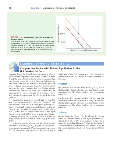
FIGURE 1.4 Comparative Statics in the Market for
Masters Badges
In a normal year, the market equilibrium occurs at the $600
intersection of D 1 and S, and the equilibrium price for
Masters badges is $1,100. The recession of 2009 caused D D
a leftward shift in the demand curve from D 1 to D 2 , 2 1
and the market equilibrium price of Masters badges Quantity (number of Masters badges)
fell to $600.

LEARNING-BY-DOING EXERCISE 1.3
S
D
E
Comparative Statics with Market Equilibrium in the
U.S. Market for Corn
Suppose that in the United States the quantity of corn small part of the U.S. economy, so that national in-
d
demanded Q depends on two things: the price of corn come is not noticeably affected by events in the market
P and the level of income in the nation I. Assume that for corn.
the demand curve for corn is downward sloping, so
that more corn will be demanded when the price of Problem
corn is lower. Assume also that the demand curve
shifts to the right if income rises (i.e., higher income (a) Suppose that income rises from I 1 to I 2 . On a
increases the demand for corn). The dependence of clearly labeled graph, illustrate how the change in this
the quantity of corn demanded on the price of corn exogenous variable affects each of the endogenous
and income is represented by the demand function variables.
d
Q (P, I ). (b) Suppose that income remains at I 1 but that the
s
Suppose the quantity of corn offered for sale, Q , amount of rainfall increases from r 1 to r 2 . On a second
also depends on two things: the price of corn, P, and clearly labeled graph, illustrate how the change in this
the amount of rain that falls during the growing sea- exogenous variable affects each of the endogenous
son, r. The supply curve is upward sloping, so that as variables.
the price of corn rises, more corn will be offered for
sale. Assume that the supply curve shifts to the right Solution
(more corn is produced) if there is more rain. The re-
lationship showing the quantity of corn supplied at (a) As shown in Figure 1.5, the change in income
any price and amount of rainfall is the supply function shifts the demand curve to the right (increases de-
s
Q (P, r). mand), from D 1 to D 2 . The location of the supply
s
In equilibrium the price of corn will adjust so that curve, S 1 , is unaffected because Q does not depend on I.
s
d
*
*
the market will clear (Q Q ). Let’s call the equilib- The equilibrium price therefore rises from P 1 to P 2 . So
rium quantity exchanged Q* and the equilibrium price the change in income leads to a change in equilibrium
P *. We can assume that the market for corn is only a price.