Page 505 - Microeconomics, Fourth Edition

c11monopolyandmonopsony.qxd 7/14/10 7:58 PM Page 479

11.7 MONOPSONY 479

ME L
Labor
supply curve
Wage rate, w (dollars per hour of labor) Perfectly $12 A G
w(L)

B
F
competitive
wage
C
Monopsony
wage
$8
D
E
MRP L

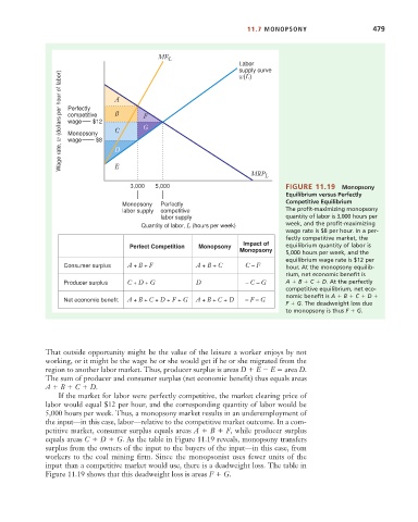
3,000 5,000 FIGURE 11.19 Monopsony
Equilibrium versus Perfectly
Competitive Equilibrium
Monopsony Perfectly
labor supply competitive The profit-maximizing monopsony
labor supply quantity of labor is 3,000 hours per
Quantity of labor, L (hours per week) week, and the profit-maximizing
wage rate is $8 per hour. In a per-
fectly competitive market, the
Impact of
Perfect Competition Monopsony equilibrium quantity of labor is
Monopsony 5,000 hours per week, and the
equilibrium wage rate is $12 per
Consumer surplus A + B + F A + B + C C – F hour. At the monopsony equilib-
rium, net economic benefit is
Producer surplus C + D + G D – C – G A B C D. At the perfectly
competitive equilibrium, net eco-
Net economic benefit A + B + C + D + F + G A + B + C + D – F – G nomic benefit is A B C D
F G. The deadweight loss due
to monopsony is thus F G.

That outside opportunity might be the value of the leisure a worker enjoys by not
working, or it might be the wage he or she would get if he or she migrated from the
region to another labor market. Thus, producer surplus is areas D E E area D.
The sum of producer and consumer surplus (net economic benefit) thus equals areas
A B C D.
If the market for labor were perfectly competitive, the market clearing price of
labor would equal $12 per hour, and the corresponding quantity of labor would be
5,000 hours per week. Thus, a monopsony market results in an underemployment of
the input—in this case, labor—relative to the competitive market outcome. In a com-
petitive market, consumer surplus equals areas A B F, while producer surplus
equals areas C D G. As the table in Figure 11.19 reveals, monopsony transfers
surplus from the owners of the input to the buyers of the input—in this case, from
workers to the coal mining firm. Since the monopsonist uses fewer units of the
input than a competitive market would use, there is a deadweight loss. The table in
Figure 11.19 shows that this deadweight loss is areas F G.