Page 235 - Economics

CONFIRMING PAGES

206 CHAPTER TEN APPENDIX

• Finally, suppose the price level rises from P to P . FIGURE 2 Shifts in the aggregate expenditures
2
3
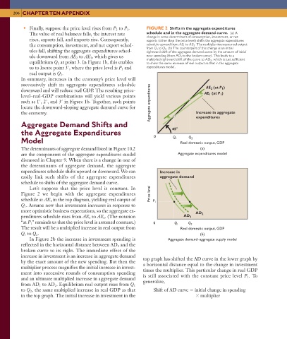
The value of real balances falls, the interest rate schedule and in the aggregate demand curve. (a) A
change in some determinant of consumption, investment, or net
rises, exports fall, and imports rise. Consequently, exports (other than the price level) shifts the aggregate expenditures
the consumption, investment, and net export sched- schedule upward from AE 1 to AE 2 . The multiplier increases real output
from Q 1 to Q 2 . (b) The counterpart of this change is an initial
ules fall, shifting the aggregate expenditures sched- rightward shift of the aggregate demand curve by the amount of initial
ule downward from AE to AE , which gives us new spending (from AD 1 to the broken curve). This leads to a
3
2
multiplied rightward shift of the curve to AD 2 , which is just sufficient
equilibrium Q at point 3. In Figure 1b, this enables to show the same increase of real output as that in the aggregate
3
us to locate point 3 , where the price level is P and expenditures model.
3
real output is Q .
3
In summary, increases in the economy’s price level will
successively shift its aggregate expenditures schedule AE 2 (at P 1 )
downward and will reduce real GDP. The resulting price- AE 1 (at P 1 )
level–real-GDP combinations will yield various points
such as 1 , 2 , and 3 in Figure 1b. Together, such points Aggregate expenditures
locate the downward-sloping aggregate demand curve for
the economy. Increase in aggregate
expenditures
Aggregate Demand Shifts and
45
the Aggregate Expenditures
0 Q 1 Q 2
Model Real domestic output, GDP
The determinants of aggregate demand listed in Figure 10.2 (a)
are the components of the aggregate expenditures model Aggregate expenditures model
discussed in Chapter 9. When there is a change in one of
the determinants of aggregate demand, the aggregate
expenditures schedule shifts upward or downward. We can Increase in
easily link such shifts of the aggregate expenditures aggregate demand
schedule to shifts of the aggregate demand curve.
Let’s suppose that the price level is constant. In
Figure 2 we begin with the aggregate expenditures Price level
schedule at AE in the top diagram, yielding real output of P 1
1
Q . Assume now that investment increases in response to
1
more optimistic business expectations, so the aggregate ex-
AD 2
penditures schedule rises from AE to AE . (The notation AD 1
1
2
“at P ” reminds us that the price level is assumed constant.) 0 Q 1 Q 2
1
The result will be a multiplied increase in real output from Real domestic output, GDP
Q to Q . (b)
2
1
In Figure 2b the increase in investment spending is Aggregate demand–aggregate supply model
reflected in the horizontal distance between AD and the
1
broken curve to its right. The immediate effect of the
increase in investment is an increase in aggregate demand top graph has shifted the AD curve in the lower graph by
by the exact amount of the new spending. But then the a horizontal distance equal to the change in investment
multiplier process magnifies the initial increase in invest- times the multiplier. This particular change in real GDP
ment into successive rounds of consumption spending is still associated with the constant price level P . To
and an ultimate multiplied increase in aggregate demand generalize, 1
from AD to AD . Equilibrium real output rises from Q
1
1
2
to Q , the same multiplied increase in real GDP as that Shift of AD curve initial change in spending
2
in the top graph. The initial increase in investment in the multiplier

8/21/06 4:51:13 PM
mcc26632_ch10_187-207.indd 206 8/21/06 4:51:13 PM
mcc26632_ch10_187-207.indd 206