Page 234 - Economics

CONFIRMING PAGES

CHAPTER TEN APPENDIX 205

The Relationship of the Aggregate

Demand Curve to the Aggregate

Expenditures Model*

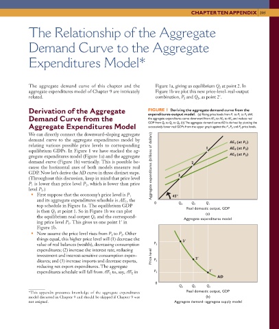
The aggregate demand curve of this chapter and the Figure 1a, giving us equilibrium Q at point 2. In
2
aggregate expenditures model of Chapter 9 are intricately Figure 1b we plot this new price-level–real-output
related. combination, P and Q , as point 2 .
2
2
Derivation of the Aggregate FIGURE 1 Deriving the aggregate demand curve from the
expenditures-output model. (a) Rising price levels from P 1 to P 2 to P 3 shift
Demand Curve from the the aggregate expenditures curve downward from AE 1 to AE 2 to AE 3 and reduce real
GDP from Q 1 to Q 2 to Q 3 . (b) The aggregate demand curve AD is derived by plotting the
Aggregate Expenditures Model successively lower real GDPs from the upper graph against the P 1 , P 2 , and P 3 price levels.
We can directly connect the downward-sloping aggregate
demand curve to the aggregate expenditures model by AE 1 (at P 1 )
relating various possible price levels to corresponding 1
equilibrium GDPs. In Figure 1 we have stacked the ag- AE 2 (at P 2 )
gregate expenditures model (Figure 1a) and the aggregate AE 3 (at P 3 )
demand curve (Figure 1b) vertically. This is possible be- 2
cause the horizontal axes of both models measure real Aggregate expenditures (billions of dollars)
GDP. Now let’s derive the AD curve in three distinct steps. 3
(Throughout this discussion, keep in mind that price level
P is lower than price level P , which is lower than price
2
1
level P .)
3
• First suppose that the economy’s price level is P 45
1
and its aggregate expenditures schedule is AE , the 0
1
top schedule in Figure 1a. The equilibrium GDP Q 3 Q 2 Q 1
is then Q at point 1. So in Figure 1b we can plot Real domestic output, GDP
1
(a)
the equilibrium real output Q and the correspond- Aggregate expenditures model
1
ing price level P . This gives us one point 1 in
1
Figure 1b.
• Now assume the price level rises from P to P . Other
1
2
things equal, this higher price level will (1) decrease the 3
value of real balances (wealth), decreasing consumption P 3
expenditures; (2) increase the interest rate, reducing
investment and interest-sensitive consumption expen- Price level
ditures; and (3) increase imports and decrease exports, P 2 2
reducing net export expenditures. The aggregate
expenditures schedule will fall from AE to, say, AE in P 1 1
1
2
AD
0
Q 3 Q 2 Q 1
*This appendix presumes knowledge of the aggregate expenditures Real domestic output, GDP
model discussed in Chapter 9 and should be skipped if Chapter 9 was (b)
not assigned. Aggregate demand–aggregate supply model

8/21/06 4:51:12 PM
mcc26632_ch10_187-207.indd 205 8/21/06 4:51:12 PM
mcc26632_ch10_187-207.indd 205