Page 101 - ISCI’2017

The noise implementations ( ) tξ are also a continuous function of time. Continuous channel capacity

is defined in [2] as the maximum (over all possible input distributions) of the function which

essentially similar to the expression (1):

1  
(
C =  2FT max { HY − ( ) HY X )} , (10)
⋅
T  f (x) 
where F – the frequency band which restricts the channel; T – duration of channel output
observation; 2FT – number of degrees of freedom, defined on the duration T, as the number of

independent measurements of function with a limited spectrum, defined by the sampling theorem
[1,2]. In the formula (10) H(Y) – denotes the channel output entropy, and conditional entropy

H(YX) defined by the expression (7). The difference, the maximum of which is sought in (10), is

usually referred to as the average mutual information between the input and output per one channel
usage:

∞∞ ( f x, y )
)
( I X,Y = ) HY − ( ) HY X = ( ) ∫∫ ( f x, y log . (11)
( ) ( ) y
−∞ −∞ f xf
Then for one channel usage:

C = max ( {I X,Y )} . (12)
f (x)

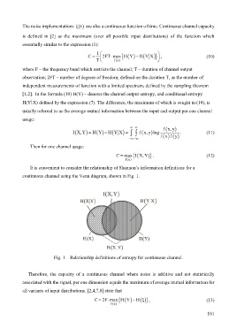
It is convenient to consider the relationship of Shannon’s information definitions for a
continuous channel using the Venn diagram, shown in Fig. 1.

Fig. 1 – Relationship definitions of entropy for continuous channel.

Therefore, the capacity of a continuous channel where noise is additive and not statistically
associated with the signal, per one dimension equals the maximum of average mutual information for

all variants of input distributions. [2,4,7,8] state that

ξ
( ) H−
C 2F max= ⋅ {H Y ( )} , (13)
f (x)
101