Page 28 - Fiber Optic Communications Fund

Electromagnetics and Optics 9

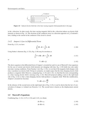
Conductor

y
B=B z z
E x
x
+ –
Figure 1.8 Induced electric field due to the time-varying magnetic field perpendicular to the page.

in the z-direction. In other words, the time-varying magnetic field in the z-direction induces an electric field
intensity as shown in Fig. 1.8. The electrons in the conductor move in a direction opposite to E (Coulomb’s
x
law), leading to the current in the conductor if the circuit is closed.

1.4.2 Ampere’s Law in Differential Form

From Eq. (1.21), we have
H ⋅ dl = J ⋅ dS. (1.40)
∮ ∫
L 1 S
Using Stokes’s theorem (Eq. (1.32)), Eq. (1.40) may be rewritten as

(∇ × H) ⋅ dS = J ⋅ dS (1.41)
∫ ∫
S S
or
∇× H = J. (1.42)
The above equation is the differential form of Ampere’s circuital law and it is one of Maxwell’s four equations
for the case of current and electric field intensity not changing with time. Eq. (1.40) holds true only under
non-time-varying conditions. From Faraday’s law (Eq. (1.34)), we see that if the magnetic field changes with
time, it produces an electric field. Owing to symmetry, we might expect that the time-changing electric field
produces a magnetic field. However, comparing Eqs. (1.34) and (1.42), we find that the term corresponding
to a time-varying electric field is missing in Eq. (1.42). Maxwell proposed adding a term to the right-hand
side of Eq. (1.42) so that a time-changing electric field produces a magnetic field. With this modification,
Ampere’s circuital law becomes
D
∇× H = J + . (1.43)
t
In the absence of the second term on the right-hand side of Eq. (1.43), it can be shown that the law of con-
servation of charges is violated (see Exercise 1.4). The second term is known as the displacement current
density.

1.5 Maxwell’s Equations
Combining Eqs. (1.12), (1.27), (1.34) and (1.43), we obtain

div D = , (1.44)
div B = 0, (1.45)