Page 72 - ansys

4.1.3 CFD Process

The entire CFD process consists of three stages: pre-processing, solving, and post-processing. These
are diagrammed in Figure 1.1.

Figure 4.1 The computational fluid dynamics process.
All three processes are interdependent. As much as 90% of effort is used in the meshing
(preprocessing) stage. This requires the user to be dexterous and there must be the idea of creating an
understandable topology. The next stage is to solve the governing equations of flow, which is the com-
puter's work. Remember that an error embedded in the mesh will prop-agate in the solving stage as
well, and if you are lucky enough, you may get a converged solution. However, mostly, owing to only
one culprit cell, the solution diverges. The next phase after solving equations is post-processing.
There, the results of whatever was input and solved are obtained; colorful pictures showing contours
are interpreted for product design, development, or optimization. For validation, the results are
compared with experimental data. If any experimental data are absent, the grid convergence study
better judges the authenticity of the results. In that case, the mesh is refined two or three times, each
time solving and getting results, until a never-changing result (asymptotically converged solution) is
obtained.
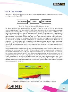
Post-processing has its own delights, and you can impress people by showing flow simulations such as
path lines, flow contours, vector plots, flow ribbons, cylinders, and so forth. In unsteady flows, such as
for direct numerical simulation (DNS) and large eddy simulation (LES), the iso-surface of Q-criterion
or l-criterion is also shown sometimes. Post-processing software such as Tecplot has the ability to see
multiple things simultaneously in a single picture. As examples, the stream line and flow contours are
shown simultaneously in Figure 1.2 for Ariane5 base flow and Figure 1.3 shows the flow over a delta
wing. There, the iso-surface of constant pressure is shown over the wing, which is colored by the Mach
number. An iso-surface is a surface formed by a collection of points with the same value of a property
(such as temperature pressure).

Figure 4.2 Flow structure at the base of Ariane5 ESA Satellite Launch Vehicle

65