Page 27 - VIRANSH COACHING CLASSES

which is based on table 3.1 the demand of all consumers at various prices.
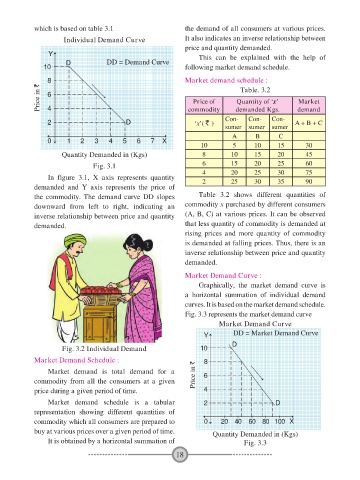
Individual Demand Curve It also indicates an inverse relationship between
price and quantity demanded.
Y This can be explained with the help of
D DD = Demand Curve
10 following market demand schedule.

8 Market demand schedule :
Price in ` 6 Price of Quantity of ‘x’ Market
Table. 3.2

4
demanded Kgs.
commodity
Con- Con- Con- demand
2 D ‘x’( ` ) A + B + C
sumer sumer sumer
A B C
0 1 2 3 4 5 6 7 X
10 5 10 15 30
Quantity Demanded in (Kgs) 8 10 15 20 45

Fig. 3.1 6 15 20 25 60
4 20 25 30 75
In figure 3.1, X axis represents quantity 2 25 30 35 90
demanded and Y axis represents the price of
the commodity. The demand curve DD slopes Table 3.2 shows different quantities of
downward from left to right, indicating an commodity x purchased by different consumers
inverse relationship between price and quantity (A, B, C) at various prices. It can be observed
demanded. that less quantity of commodity is demanded at
rising prices and more quantity of commodity
is demanded at falling prices. Thus, there is an
inverse relationship between price and quantity
demanded.

Market Demand Curve :
Graphically, the market demand curve is
a horizontal summation of individual demand
curves. It is based on the market demand schedule.
Fig. 3.3 represents the market demand curve
Market Demand Curve
DD = Market Demand Curve
Y
Fig. 3.2 Individual Demand 10 D

Market Demand Schedule : 8
Market demand is total demand for a Price in ` 6
commodity from all the consumers at a given
price during a given period of time. 4
Market demand schedule is a tabular 2 D
representation showing different quantities of
commodity which all consumers are prepared to 0 20 40 60 80 100 X
buy at various prices over a given period of time. Quantity Demanded in (Kgs)
It is obtained by a horizontal summation of Fig. 3.3

18