Page 206 - Six Sigma Advanced Tools for Black Belts and Master Black Belts

OTE/SPH
OTE/SPH
Char Count= 0
August 31, 2006
2:58
JWBK119-12
Logistic Regression Approach 191
have been proposed in literature. Algorithms that are similar to backward elimination
and forward selection procedures in ordinary linear regression have been proposed.
Criteria used in these algorithms include statistics such as the Akaike information
criterion (AIC) and others based on the difference in likelihood ratios. In this chap-
ter, we introduce a very simplistic backward elimination process which utilizes the
difference in the likelihood ratios of two possible models. For model selection proce-
dures using such measures, one of the models in the comparison must be a special
case of the other. Assuming the likelihood ratio evaluated with equation (12.16) of the
more complex model is given by G 1 and that of the simpler model is given by G 2 ,a
hypothesis test can be conducted on the difference between these likelihood ratios,
G D = G 1 − G 2 . Under the assumed models and specified hypothesis test, these dif-
2
ferences typically follow an approximate null χ distribution with degrees of freedom
equivalent to the difference in degrees of freedom associated with the likelihood ratios
of each model compared. Any significant difference indicates the need for additional
variables in achieving a more predictive model. On the other hand, if there are no
significant differences, the additional complexity that accompanies the more complex
model is deemed unnecessary. Such a likelihood ratio statistic can implemented in a
backward elimination procedure. The horseshoe crab example is used to demonstrate
this backward elimination procedure.
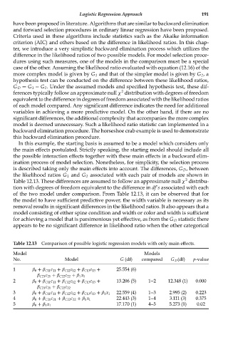
In this example, the starting basis is assumed to be a model which considers only
the main effects postulated. Strictly speaking, the starting model should include all
the possible interaction effects together with these main effects in a backward elim-
ination process of model selection. Nonetheless, for simplicity, the selection process
is described taking only the main effects into account. The differences, G D , between
the likelihood ratios G 1 and G 2 associated with each pair of models are shown in
2
Table 12.13. These differences are assumed to follow an approximate null χ distribu-
tion with degrees of freedom equivalent to the difference in df’s associated with each
of the two model under comparison. From Table 12.13, it can be observed that for
the model to have sufficient predictive power, the width variable is necessary as its
removal results in significant differences in the likelihood ratios. It also appears that a
model consisting of either spine condition and width or color and width is sufficient
for achieving a model that is parsimonious yet effective, as from the G D statistic there
appears to be no significant difference in likelihood ratio when the other categorical

Table 12.13 Comparison of possible logistic regression models with only main effects.

Model Models
No. Model G (df) compared G D (df) p-value
1 β 0 + β C11 c 11 + β C12 c 12 + β C13 c 13 + 25.554 (6)
β C21 c 21 + β C22 c 22 + β 1 x 1
2 β 0 + β C11 c 11 + β C12 c 12 + β C13 c 13 + 13.206 (5) 1--2 12.348 (1) 0.000
β C21 c 21 + β C22 c 22
3 β 0 + β C11 c 11 + β C12 c 12 + β C13 c 13 + β 1 x 1 22.559 (4) 1--3 2.995 (2) 0.223
4 β 0 + β C21 c 21 + β C22 c 22 + β 1 x 1 22.443 (3) 1--4 3.111 (3) 0.375
5 β 0 + β 1 x 1 17.170 (1) 4--5 5.273 (1) 0.02