Page 398 - Six Sigma Advanced Tools for Black Belts and Master Black Belts

OTE/SPH
OTE/SPH
Char Count= 0
August 31, 2006
JWBK119-25
3:9
Backward CUSUM 383
follows (Harrison and Davies 16 ):
S 1 = e t ,
S 2 = e t + e t−1 ,
S 3 = e t + e t−1 + e t−2 , etc.
These quantities are called backward cumulative sums or BCUSUMs. In applying
this scheme, if we have, say, n observations or forecast errors, we need to calculate n
sums. The monitoring is done on a real-time basis, thus n increases as the number of
observations increases. In a typical forecasting activity, we are only interested in the
first few values of S. Thus, most authors, particularly those dealing with short-term
forecasting, suggest the use of the following BCUSUMs: 17,18
S t,1 = e t , t = 1, 2,..., m,
S t,2 = e t + e t−1 , t = 2, 3,..., m,
...
S t,m = e t + e t−1 +· · · + e t−m+1 , t = m,
where e 1 , e 2 , . .., e m represent the latest m forecast errors being tracked. To determine
whether the system is in control, Harrison and Davies 16 proposed establishing the
control limits L 1 , L 2 , . .., L 6 for the last six BCUSUMs (i.e., S t,1 , S t,2 ,. . . , S t,6 ). As long
as these are within the specified control limits, the system is deemed in control or
stable. Since the variance of the partial sums increases as the number of errors being
summed increases, we can expect that L 1 < L 2 < ··· < L 6 . Harrison and Davies 16
suggested the use of the following equation for calculating the control limits:
L i = σ ε w(i + h),
where σ ε represents the standard deviation of the errors, and w and h are parameters
to be chosen. One typically selects the values of w and h using simulation.
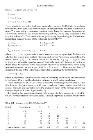
To illustrate how a BCUSUM works, we use the example given by Gardner. 19 For
this data set, the parameters σ ε = 10,w = 1, and h = 2 were used to establish the
control limits. In the example below, the change in mean of the forecast errors was
detected in period 6 when S 6,2 exceeded L 2 .
Recognizing that forecast monitoring is done sequentially, one can easily see that Ta-
ble 25.1 contains unnecessary calculations. The only important information for control

Table 25.1 Example of the BCUSUM method. 19

Period Forecast error S 1 S 2 S 3 S 4 S 5 S 6
1 −10 −10
2 20 20 10
3 15 15 35 25
4 5 5 20 40 30
5 −25 −25 −20 −5 15 5
6 −25 −25 −50 −45 −30 −10 −20
±30 ±40 ±50 ±60 ±70 ±80
Control limits:L 1 to L 6