Page 402 - Six Sigma Advanced Tools for Black Belts and Master Black Belts

OTE/SPH
OTE/SPH
Char Count= 0
August 31, 2006
JWBK119-25
3:9
Symmetric Cumulative Sum Schemes 387
Similar to the one-sided monitoring scheme, the z* for equations (25.9) and (25.10) is
chosen such that the in-control ARL is equivalent to some pre-specified value.
25.3 SYMMETRIC CUMULATIVE SUM SCHEMES

The BCUSUM scheme discussed earlier is computationally intensive. Interestingly,
we can translate the BCUSUM scheme into an equivalent CUSUM representation.
The following characteristics of symmetric functions are important in establishing a
CUSUM scheme based on the UMP test. Let y = f 1 (t) and y = f 2 (t) represent two
real functions of t.If f 1 (t) and f 2 (t) are symmetric about y = 0, then f 1 (t) =− f 2 (t). In
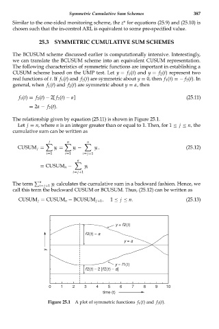
general, when f 1 (t) and f 2 (t) are symmetric about y = a, then

f 1 (t) = f 2 (t) − 2[ f 2 (t) − a] (25.11)
= 2a − f 2 (t).

The relationship given by equation (25.11) is shown in Figure 25.1.
Let j = n, where n is an integer greater than or equal to 1. Then, for 1 ≤ j ≤ n, the
cumulative sum can be written as
j n n

CUSUM j = y i = y i − y i , (25.12)
i=1 i=1 i= j+1
n

= CUSUM n − y i
i= j+1
n

The term y i calculates the cumulative sum in a backward fashion. Hence, we
i= j+1
call this term the backward CUSUM or BCUSUM. Thus, (25.12) can be written as
CUSUM j = CUSUM n − BCUSUM j+1 , 1 ≤ j ≤ n. (25.13)

y = f2(t)
f2(t) − a
y = a
y

y = f1(t)
f2(t) − 2 [f2(t) − a]

0 1 2 3 4 5 6 7 8 9 10
time (t)
Figure 25.1 A plot of symmetric functions f 1 (t) and f 2 (t).