Page 404 - Six Sigma Advanced Tools for Black Belts and Master Black Belts

OTE/SPH
OTE/SPH
3:9
August 31, 2006
Char Count= 0
JWBK119-25
Symmetric Cumulative Sum Schemes 389
Table 25.2 Calculation of CUSUM and BCUSUM with the corresponding masks.
Time ( j) Observation y j BCUSUM j CUSUM j BCUSUM mask CUSUM mask
1 0.54 10.08 0.54 12.55 −2.04
2 −1.20 9.54 −0.66 12.12 −1.60
3 2.20 10.74 1.54 11.68 −1.14
4 −1.24 8.54 0.30 11.22 −0.67
5 −0.56 9.78 −0.26 10.75 −0.17
6 1.30 10.34 1.04 10.25 0.36
7 −0.02 9.04 1.02 9.72 0.92
8 0.14 9.06 1.16 9.16 1.51
9 0.16 8.92 1.32 8.57 2.14
10 0.86 8.76 2.18 7.94 2.84
11 0.92 7.90 3.10 7.24 3.60
12 2.40 6.98 5.50 6.48 4.47
13 3.08 4.58 8.58 5.61 5.50
14 0.26 1.50 8.84 4.58 6.84
15 1.24 1.24 10.08 3.24 10.08

For comparison purposes, the control chart parameters are chosen such that the in-
controlARLfortheone-sidedschemeisapproximately470.Asexpected,theBCUSUM
and CUSUM with parabolic mask give similar ARL performance. From the table, it
is clear that for a shift in mean below 0.5 σ and greater than 1.5σ, the CUSUM with
parabolic mask gives the best ARL performance. The CUSUM with V-mask is superior
only in tracking down shifts it is designed to detect (i.e., 2k). The Shewhart CUSUM
scheme 25 is an improvement on the sensitivity of the equivalent V-mask scheme but
it is still less sensitive compared to a CUSUM with a parabolic, Bissell or snub-nosed
mask.

15
upper BCUSUM mask arm BCUSUM

CUSUM(t =15) CUSUM
10
Cumulative Sum 5 CUSUM(t =15) /2

0

lower CUSUM mask arm
−5
0 2 4 6 8 10 12 14
Time Period ( j)
23
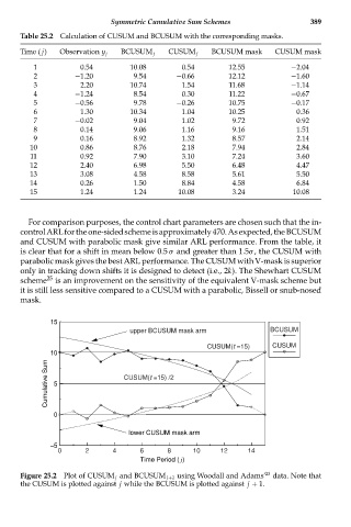
Figure 25.2 Plot of CUSUM j and BCUSUM j+1 using Woodall and Adams’ data. Note that
the CUSUM is plotted against j while the BCUSUM is plotted against j + 1.