Page 408 - Six Sigma Advanced Tools for Black Belts and Master Black Belts

OTE/SPH
OTE/SPH
3:9
Char Count= 0
JWBK119-25
August 31, 2006
CUSUM Scheme for Autocorrelated Observations 393
0
will signal a change when y 1 > z * υ 1 . The assumption that CUSUM = 0 is crucial to
0
the use of the V-mask in which the initial observation is used in decision making
applies only when initial CUSUM value is zero and for a stationary process with a
zero mean. When the process is not centered at zero, one monitors the following the
following CUSUM scheme:
j

n
CUSUM = (y i − μ 0 ) ,
j
i=1
where μ 0 represents the mean of the process.
25.4.3 Sensitivity analysis
In analyzing the performance of the proposed CUSUM scheme, we focus our attention
on the detection of changes in the mean of an AR(1) process. The importance of an
AR(1) process in SPC has been emphasized in the literature. 8,11,12 In the following, we
describe a simple graphical procedure that can facilitate the choice of the constraint
z * . Subsequently, we compare the performance of the proposed CUSUM scheme with
the other established procedures for monitoring autocorrelated processes. We then
address one of the major criticisms in implementing a CUSUM in mask form (i.e. how
far should we extend the CUSUM mask arms?).

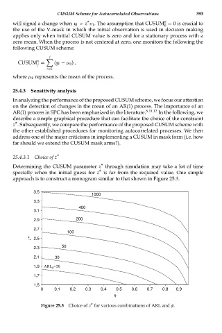
25.4.3.1 Choice of z *
Determining the CUSUM parameter z * through simulation may take a lot of time
specially when the initial guess for z * is far from the required value. One simple
approach is to construct a monogram similar to that shown in Figure 25.3.

3.5
1000
3.3
400
3.1
2.9 200
2.7
100
z* 2.5
2.3 50
2.1 30
1.9 ARL 0 =20
1.7

1.5
0 0.1 0.2 0.3 0.4 0.5 0.6 0.7 0.8 0.9
φ

Figure 25.3 Choice of z* for various combinations of ARL and φ.