Page 47 - Prosig Catalogue 2005

SOFTWARE PRODUCTS
FOURIER ANALYSIS - THE BASICS AND BEYOND

If we have data taken over a longer period then the frequency spacing will to cancel during the second part. The same of course happens in reverse
be narrower. In many cases this will minimize the problem, but if there is around those frequencies close to 192Hz.
no exact match the same phenomenon will arise.
Another example is where a signal is extended by zeroes. Again the
Fourier analysis tells us the amplitude and phase of that set of cosines amplitude is reduced. In this case the reduction is proportional to the
which have the same duration as the original signal. Suppose now we percentage extension by zeroes.
take a signal which again is composed of unit amplitude 64Hz sine wave
and a 0.25 amplitude 192Hz sine wave signals but this time the 64Hz The important point to note is that the Fourier analysis assumes that the
signal occupies the first half and the 192Hz signal occupies the second sines and cosines last for the entire duration.
half. That is we now have a one second signal as shown below. Swept Sine Signal Training & Support
With a swept sine signal theoretically each frequency only lasts for an
instant in time. A swept sine signal sweeping from 10Hz to 100Hz is
shown below.

Condition Monitoring

Figure 8. Two sines joined
The result of an FFT of these two joined signals is shown below.
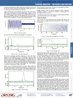
Figure 11 Swept sine, unit amplitude, !0 to 100Hz.

Software

Figure 12 FFT of Swept Sine

This has 512 points at 1024 samples/second. Thus the sweep rate was
Figure 9 FFT of two joined sinewaves 180Hz/second. The FFT of that signal shows an amplitude of about
0.075. Over the duration of the sweep the phase goes from around zero
There are, as expected, significant frequencies at 64Hz and 192Hz. to -2000° and then settles to -180° above 100Hz. If the sweep rate
However the half amplitudes are now 0.25 (instead of 0.5) and 0.0625 is lowered to around 10Hz/second then the amplitude becomes about
(instead of 0.125). One interpretation of what the FFT is telling us is that 0.019. The relationship between the spectrum level the amplitude and
there is a cosine wave at 64Hz of half amplitude 0.25 for the whole one sweep rate of the original swept sine is not straight forward.
second duration and another one of half amplitude 0.0625 for the whole
duration. But we know that we had a 64Hz signal with a half amplitude of It is clear that one has to interpret a simple Fourier analysis, whether it is
0.5 for the first part of the time and a 192Hz signal with a half amplitude done by an FFT or by a DFT, with some care. A Fourier analysis shows the
of 0.125 for the second part. What is happening? (half) amplitudes and phases of the constituent cosine waves that exist
for the whole duration of that part of the signal that has been analyzed.
A closer look at the spectrum around 64Hz as shown below reveals that Although we have not discussed it, a Fourier analyzed signal is invertible. Hardware
we have a large number of frequencies around 64Hz. This time they are That is if we have the Fourier analysis over the entire frequency range
1Hz apart as we had one second of data. Their relative amplitudes and from zero to half sample rate then we may do an inverse Fourier transform
phases combine to double the amplitude at 64Hz over the first part and to get back to the time signal. One point that arises from this is that if
the signal being analyzed has some random noise in it, then so does
the Fourier transformed signal. Fourier analysis by itself does nothing to
remove or minimise the effects of noise. Thus simple Fourier analysis is
not suitable for random data, but it is for signals such as transients and
complicated or simple periodic signals such as those generated by an
engine running at a constant speed.
We have not considered Auto Spectral Density (also sometimes called
Power Spectral Density) or RMS Spectrum Level Analyses here. They are
discussed in another article. However for completeness it is worth noting
that the essential difference between ASD analysis and FFT analysis is System Packages
that ASDs are describing the distribution in frequency of the ‘power’ in the
signal whilst Fourier analysis is determining (half) amplitudes and phases.
While ASDs and RMS Spectrum Level analyses do reduce the effects of
any randomness, Fourier analysis does not. Where confusion occurs is
that both analysis methods may use FFT algorithms. This is not to do with
Figure 10. FFT (part) of joined signals the objective of the analysis or its properties but rather with efficiency of

http://prosig.com +1 248 443 2470 (USA) or contact your 47
sales@prosig.com +44 (0)1329 239925 (UK) local representative
A CMG Company