
Page 34 - Shock and Vibration Overview
P. 34
Analysis Overview
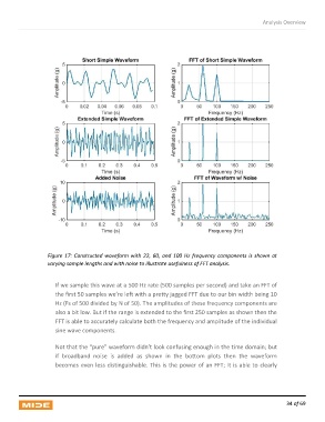
Figure 17: Constructed waveform with 22, 60, and 100 Hz frequency components is shown at
varying sample lengths and with noise to illustrate usefulness of FFT analysis.
If we sample this wave at a 500 Hz rate (500 samples per second) and take an FFT of
the first 50 samples we’re left with a pretty jagged FFT due to our bin width being 10
Hz (Fs of 500 divided by N of 50). The amplitudes of these frequency components are
also a bit low. But if the range is extended to the first 250 samples as shown then the
FFT is able to accurately calculate both the frequency and amplitude of the individual
sine wave components.
Not that the “pure” waveform didn’t look confusing enough in the time domain; but
if broadband noise is added as shown in the bottom plots then the waveform
becomes even less distinguishable. This is the power of an FFT; it is able to clearly
34 of 69