Page 346 - Mechatronics with Experiments

JWST499-Cetinkunt
JWST499-c06
332 MECHATRONICS Printer: Yet to Come October 9, 2014 8:1 254mm×178mm
Maximum for
typical device
Typical shift (high)
Output value k Output value Normal curve Output value Nominal

for typical device
1 Minimum Typical shift (low)
k for typical device

Input value Input value Input value

Downscale
Actual data trend
Output value Best linear curve fit Output value Input value

Hysteresis
Upscale
Input value Input value
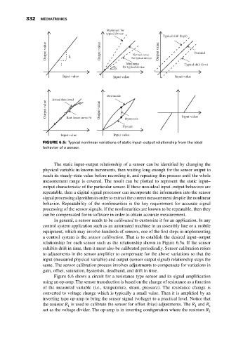
FIGURE 6.5: Typical nonlinear variations of static input–output relationship from the ideal
behavior of a sensor.

The static input–output relationship of a sensor can be identified by changing the
physical variable in known increments, then waiting long enough for the sensor output to
reach its steady-state value before recording it, and repeating this process until the whole
measurement range is covered. The result can be plotted to represent the static input–
output characteristic of the particular sensor. If these non-ideal input–output behaviors are
repeatable, then a digital signal processor can incorporate the information into the sensor
signal processing algorithm in order to extract the correct measurement despite the nonlinear
behavior. Repeatability of the nonlinearities is the key requirement for accurate signal
processing of the sensor signals. If the nonlinearities are known to be repeatable, then they
can be compensated for in software in order to obtain accurate measurement.
In general, a sensor needs to be calibrated to customize it for an application. In any
control system application such as an automated machine in an assembly line or a mobile
equipment, which may involve hundreds of sensors, one of the first steps in implementing
a control system is the sensor calibration. That is to establish the desired input–output
relationship for each sensor such as the relationship shown in Figure 6.5a. If the sensor
exhibits drift in time, then it must also be calibrated periodically. Sensor calibration refers
to adjustments in the sensor amplifier to compensate for the above variations so that the
input (measured physical variable) and output (sensor output signal) relationship stays the
same. The sensor calibration process involves adjustments to compensate for variations in
gain, offset, saturation, hysterisis, deadband, and drift in time.
Figure 6.6 shows a circuit for a resistance type sensor and its signal amplification
using an op-amp. The sensor transduction is based on the change of resistance as a function
of the measured variable (i.e., temperature, strain, pressure). The resistance change is
converted to voltage change which is typically a small value. Then it is amplified by an
inverting type op-amp to bring the sensor signal (voltage) to a practical level. Notice that
the resistor R is used to calibrate the sensor for offset (bias) adjustments. The R and R s
1
1
act as the voltage divider. The op-amp is in inverting configuration where the resistors R 2