Page 890 - Mechatronics with Experiments

876 MECHATRONICS

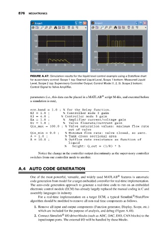
FIGURE A.47: Simulation results for the liquid level control example using a Stateflow chart
for supervisory control: Scope 1 top: Desired Liquid Level, Scope 1 bottom: Measured Liquid
Level, Scope 2 top: Supervisory Controller Output: Control Mode (1, 2, 3). Scope 2 bottom:
Control Signal to Valve Amplifier.

®
parameters (i.e., this data can be placed in a MATLAB script M-file, and executed before
a simulation is run),

err_band = 1.0 ; % for the Relay function.
K2 = 1.0 ; % Controller mode 2 gain
K3 = 4.0 ; % Controller mode 3 gain
Ka = 1.0 ; % Amplifier current/voltage gain
Kv = 1.0 ; % Valve flowrate/currrent gain
Qin_max = 100.0 ; % Valve saturation values: maximum flow rate
out of valve
Qin_min = 0.0 ; % Minimum flow rate: valve closed, so zero.
A = 1.0 ; % Tank cross sectional area
R = 10.0 ; % Outflow rate resistance as function of
liquid
% height: Q_out = (1/R) * h

Notice the change in the controller output discontinuity as the supervisory controller
switches from one controller mode to another.

A.4 AUTO CODE GENERATION

One of the most powerful, versatile, and widely used MATLAB ® features is automatic
code generation from model for a target embedded controller for real-time implementation.
The auto-code generation approach to generate a real-time code to run on an embedded
electronic control module (ECM) has already largely replaced the manual coding in C and
assembly languages in industry.
®
For a real-time implementation on a target ECM, a typical Simulink /StateFlow
algorithm should be modified to remove all non-real time components as follows.
1. Remove all input and output components (Function generator, Display, Scope, etc.)
which are included for the purpose of analysis, and debug (Figure A.48).
®
2. Connect Simulink I/O driver blocks (such as ADC, DAC, DIO, CAN blocks) to the
input/output ports. The external I/O will be handled by these blocks.