Page 143 - Servo Motors and Industrial Control Theory -

138 8 Actuators Based on Electro-Rheological Fluid

10 2000

8 6 1500

Pressure Difference 4 1000 Voltage (v)

500
2
0
0

–2
0 0.002 0.004 0.006 0.008 0.01 0.012 0.014 0.016
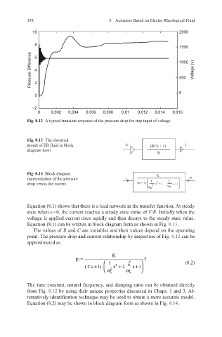
Fig. 8.12 A typical transient response of the pressure drop for step input of voltage

Fig. 8.13 The electrical
model of ER fluid in block V (RCs + 1) I
diagram form
R

Fig. 8.14 Block diagram K
representation of the pressure I  1 p
2
drop versus the current (τs + 1)  2 s + 2 ξ s + 1  
 ω n ω n 

Equation (8.1) shows that there is a lead network in the transfer function. At steady
state when s = 0, the current reaches a steady state value of V/R. Initially when the
voltage is applied current rises rapidly and then decays to the steady state value.
Equation (8.1) can be written in block diagram form as shown in Fig. 8.13.
The values of R and C are variables and their values depend on the operating
point. The pressure drop and current relationship by inspection of Fig. 8.12 can be
approximated as

p:= K I (8.2)
ξ
1
+
( s1)⋅    ω 2 n s + 2 ω n s1   
τ⋅+
2
The time constant, natural frequency, and damping ratio can be obtained directly
from Fig. 8.12 by using their unique properties discussed in Chaps. 1 and 3. Al-
ternatively identification technique may be used to obtain a more accurate model.
Equation (8.2) may be shown in block diagram form as shown in Fig. 8.14.