Page 3 - 63.2-4_49

Macchie. Data were taken from the IWEC2 (International without indoor temperature as input parameter, to better
Weather for Energy Calculations) database developed by understand the importance of this additional information.
ASHRAE within the Research Project RP-1477, As anticipated, the same analysis was carried out, at least in
“Development of 3012 Typical Year Weather Files for exploratory form, also by means of a NARX model, while
International Locations” [17], and from the Italian IGDG keeping the same basic settings in terms of training set and
dataset. In this way, two years were available in order to better method (Bayesian regularization). The delay in the network
test the predictive accuracy of the models. (the number of samples taken into account to predict each
value) was set to 3, and the number of neurons was kept at 8,
as it proved also for ANN to be a good choice.
Once the preliminary investigation was carried out, so that
the best set of input parameters was selected, a final
“incremental” test was designed in order to simulate actual
working conditions of the predictive network. In fact, under

real world conditions the amount of data to be used for training
is going to increase continuously, with the ANN dynamically
re-training as soon as new data are available. So, in order to
broaden the time horizon, a third year was added to the
simulation by repeating the EnergyPlus calculations using a
different weather file, relative to the closest station, namely
that of the city of Brindisi, 120 km south of Bari. At this point,
in order to limit the calculation burden, the ANN was re-
trained every week, gradually increasing the input dataset, and
testing its performance on the subsequent week. RMSE was
Figure 1. 3D models of the analyzed spaces representing an calculated every time in order to understand also the training
office and an industrial building time after which the ANN starts providing reliable results.

2.2 Machine learning methods

The ANN was implemented using the neural network
toolbox in Matlab [18]. To learn the parameters of the ANN
(i.e. the weights between neurons and biases) the network
training was carried out by means of a Bayesian regularization
algorithm. A two-layer feed-forward network with sigmoid
hidden neurons and linear output neurons was used. The
estimation of the number of neurons in each layer is one of the
most difficult tasks, which is generally carried out using a trial
and error procedure. In this case, 10 neurons were used as a
starting point, but they were subsequently reduced to 8, after
some testing. Daily values of partial and total energy
consumption were used as target values. Hourly values were
not considered at this stage as the fluctuations were too large,
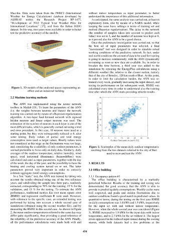
and, considering the availability of only outdoor parameters, it Figure 2. Scatterplot of the mean daily outdoor temperatures
seemed preferable to focus only on daily data. Similarly, daily resulting from the two datasets referred to the city of Bari
averages of the outdoor temperature, relative humidity, wind used to train and test the ANN
speed, total horizontal illuminance (beam+diffuse) were
calculated and used as input parameters, together with the day
of the week, the day of the year, and the possibility to have the 3. RESULTS
heating and cooling system turned on or not. The latter
parameters proved very important in order to correctly 3.1 Office building
estimate aggregate (total) energy consumptions.
In a first “static” test, the ANN was trained by taking into 3.1.1 Occupancy pattern #1
account the results obtained using one of the two reference The office building is characterized by a markedly
years, and subdividing the sample into three parts, randomly periodical behavior. Results of the training and testing sets
extracted, corresponding to 70% for the training, 15 % for the demonstrated the good accuracy that the ANN is able to
validation, and 15 % for the testing. To estimate the ANN provide in predicting daily consumptions. Weekly cycles were
performance, traditional metrics like root mean square error well respected, and peaks and sudden fluctuations due to
(RMSE) and regression coefficient R were used. However, outdoor conditions found a good match in predicted values. In
with reference to the specific case, an extended testing was quantitative terms, during the testing on the first year RMSE
performed by taking into account a whole second year of on daily consumptions was 1.8 kWh and 1.5 kWh, respectively
simulations (obtained using the second weather file), and by for the input set with and without indoor temperature.
measuring the RMSE in this second case. As shown in Figure However, when the whole second year was considered (Figure
2, the mean outdoor temperatures referred to the same day may 3), RMSE increased to 1.9 kWh for the input data with indoor
differ quite significantly, thus providing a good reference of temperature, and to 2.7 kWh for the set without it. The largest
the reliability of the predictive accuracy of the ANN. Finally, errors appeared in the reduced input dataset during the cooling
all the performance calculations were made both with and season, while both datasets had a few problems at the

454