Page 5 - 63.2-4_49

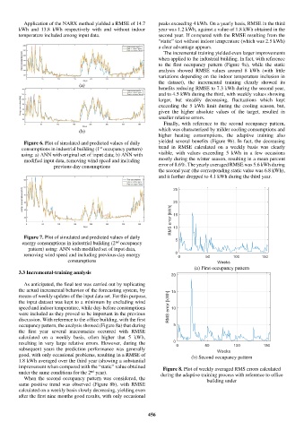
Application of the NARX method yielded a RMSE of 14.7 peaks exceeding 4 kWh. On a yearly basis, RMSE in the third
kWh and 13.8 kWh respectively with and without indoor year was 1.2 kWh, against a value of 1.8 kWh obtained in the
temperature included among input data. second year. If compared with the RMSE resulting from the
“static” test without indoor temperature (which was 2.5 kWh)
a clear advantage appears.
The incremental training yielded even larger improvements
when applied to the industrial building. In fact, with reference
to the first occupancy pattern (Figure 9a), while the static
analysis showed RMSE values around 8 kWh (with little
variations depending on the indoor temperature inclusion in
the dataset), the incremental training clearly showed its
(a)
benefits reducing RMSE to 7.3 kWh during the second year,
and to 4.5 kWh during the third, with weekly values showing
larger, but steadily decreasing, fluctuations which kept
exceeding the 5 kWh limit during the cooling season, but,
given the higher absolute values of the target, resulted in
smaller relative errors.
Finally, with reference to the second occupancy pattern,

(b) which was characterized by milder cooling consumptions and
higher heating consumptions, the adaptive training also
Figure 6. Plot of simulated and predicted values of daily yielded several benefits (Figure 9b). In fact, the decreasing
st
consumptions in industrial building (1 occupancy pattern) trend in RMSE calculated on a weekly basis was clearly
using: a) ANN with original set of input data; b) ANN with visible, with values exceeding 5 kWh in a few occasions
modified input data, removing wind speed and including mostly during the winter season, resulting in a mean percent
previous-day consumptions error of 8.6%. The yearly averaged RMSE was 5.6 kWh during
the second year (the corresponding static value was 6.8 kWh),
and it further dropped to 4.1 kWh during the third year.

Figure 7. Plot of simulated and predicted values of daily
nd
energy consumptions in industrial building (2 occupancy
pattern) using: ANN with modified set of input data,
removing wind speed and including previous-day energy
consumptions
(a) First occupancy pattern
3.3 Incremental-training analysis

As anticipated, the final test was carried out by replicating
the actual incremental behavior of the forecasting system, by
means of weekly updates of the input data set. For this purpose,
the input dataset was kept to a minimum by excluding wind
speed and indoor temperature, while day-before consumptions
were included as they proved to be important in the previous
discussion. With reference to the office building, with the first
occupancy pattern, the analysis showed (Figure 8a) that during
the first year several inaccuracies occurred with RMSE
calculated on a weekly basis, often higher that 5 kWh,
resulting in very large relative errors. However, during the
subsequent years the prediction performance was generally
good, with only occasional problems, resulting in a RMSE of (b) Second occupancy pattern
1.8 kWh averaged over the third year (showing a substantial
improvement when compared with the “static” value obtained Figure 8. Plot of weekly averaged RMS errors calculated
nd
under the same conditions for the 2 year). during the adaptive training process with reference to office
When the second occupancy pattern was considered, the building under
same positive trend was observed (Figure 8b), with RMSE
calculated on a weekly basis slowly decreasing, yielding even
after the first nine months good results, with only occasional

456