Page 4 - 63.2-4_49

beginning of the heating season in autumn. The analysis with 3.2 Industrial building
the NARX method (Figure 4), yielded a significantly worse
performance, with RMSE raising to about 4.4 kWh when 3.2.1 Occupancy pattern #1
applied to the “second” test year, independent of the input data The industrial building offered a completely different
set used. pattern of energy use, showing no variation between weekdays
and weekends in terms of equipment, thus providing a constant
3.1.2 Occupancy pattern #2 term which somewhat stabilized fluctuations particularly
nd
When the 2 occupancy pattern was used, results were during intermediate seasons (Figure 6). Given the volume of
better than those obtained with the first one. In quantitative the space and the high ventilation rate, significant heating and,
terms, during the testing on the first year RMSE was 1.0 kWh particularly, cooling loads, were observed despite the reduced
and 1.2 kWh, respectively for the input set with and without setpoint temperature in winter. Cooling loads, were clearly
indoor temperature. However, when the second year was influenced by the internal gains due to equipment and lighting.
considered (Figure 5), RMSE increased to 1.1 kWh for the During the testing on the first year RMSE for daily
input data with indoor temperature, and to 2.5 kWh for the set consumptions was 6.0 kWh and 3.9 kWh, respectively for the
without it. The agreement was very good, with the largest input set with and without indoor temperature. However, when
variations taking place during the cooling season. Again. the the second year was considered, RMSE increased to 17.1 kWh
use of the NARX method provided significantly worse for the input data with indoor temperature, and to 15.5 kWh
performance with errors between 4.1 and 4.9 kWh, depending for the set without it (Figure 6a). The largest errors clearly
on the input dataset. appeared during the cooling season, with the ANN
overestimating target data by 40% if the constant equipment
load was included, but the relative variation skyrocketed if the
equipment term was not included. So, in order to better
understand the nature of the problem, in the subsequent
analyses the equipment load was not included in the energy
demand (which is actually more realistic as in an industrial site
it will likely have a separate metering system). A detailed
comparison between simulated and predicted values showed
some odd behaviors like those appearing around day 240.
Among input data, only wind speed was unusually high during

those days, so training was repeated after excluding that
Figure 3. Plot of simulated and predicted values of daily parameter from the dataset. The test over the second year
consumptions for office building (1st occupancy pattern) yielded a RMSE of 10.0 kWh when using indoor temperature
nd
during 2 year and of 12.4 kWh when it was excluded.
A further improvement was obtained by including in the
input dataset the energy consumption of the previous day,
which yielded a RMSE equal to 7.8 kWh and 8.2 kWh,
respectively with and without indoor temperature. A few
significant inaccuracies remained between day 40 and day 50,
when outdoor temperatures were at a minimum. Attempts to
replace illuminance with radiation per area (assuming that a
more expensive sensor might be used on the smart pole), only
returned a small improvement with RMSE dropping to 6.5
kWh, but errors still appeared in the same days.
Even in this case, use of NARX method did not yield any

improvement but, conversely, returned a significantly
Figure 4. Plot of simulated and predicted values of daily worsened performance with RMSE raising to 12.4 kWh and to
consumptions for office building with NARX method during 16.6 respectively when indoor temperature was included or not
nd
the 2 year in the input dataset.

3.2.2 Occupancy pattern #2
The second occupancy pattern was characterized by
significantly lower equipment loads (and, hence, internal
gains). Thus, this time heating loads largely prevailed over
cooling loads. Use of the standard set of input parameters
showed the same limitations already observed in the first
occupancy pattern. In fact, RMSE was 12.6 kWh when using
indoor temperature and 12.1 kWh when it was excluded.
Replacement of wind speed with day-before energy
consumptions caused, as already observed, a large
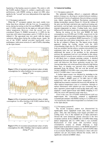
Figure 5. Plot of simulated and predicted values of daily improvement in prediction accuracy, as the RMSE dropped to
consumptions for office building (2nd occupancy pattern) 5.8 kWh when using indoor temperature, and to 6.8 kWh when
nd
during 2 year it was excluded. Replacement of illuminance values with solar
radiation rate per area barely affected the results, with no

significant variation in RMSE values.

455